

400
Practical MATLAB
® Applications for Engineers
Example 4.8
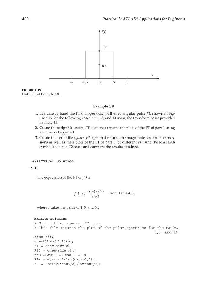
1. Evaluate by hand the FT (non-periodic) of the rectangular pulse f(t) shown in Figure 4.49 for the following cases τ = 1, 5, and 10 using the transform pairs provided
in Table 4.1.
2. Create the script fi le square_FT_num that returns the plots of the FT of part 1 using
a numerical approach.
3. Create the script fi le square_FT_sym that returns the magnitude spectrum expressions as well as their plots of the FT of part 1 for different τs using the MATLAB
symbolic toolbox. Discuss and compare the results obtained.
ANALYTICAL Solution
Part 1
The expression of the FT of f(t) is
f t
w
w
( ) ↔
sin(
)
ր
ր
2
2
(from Table 4.1)
where τ takes the value of 1, 5, and 10.
MATLAB Solution
% Script file: square _ FT _ num
% This file returns the plot of the pulse spectrums for the tau’s=
1,5, and 10
echo off;
w =-10*pi:0.1:10*pi;
F1 = ones(size(w));
F10 = ones(size(w));
tau1=1;tau5 =5;tau10 = 10;
F1= sin(w*tau1/2)./(w*tau1/2);
F5 = 5*sin(w*tau5/2)./(w*tau5/2);
−τ
0.5
f (t )
t
1.0
−τ/2
0
τ/2
τ
FIGURE 4.49
Plot of f(t) of Example 4.8.
CRC_47760_CH004.indd 400
CRC_47760_CH004.indd 400
7/28/2008 12:26:12 PM
7/28/2008 12:26:12 PM
Practical MATLAB
® Applications for Engineers
Example 4.8
1. Evaluate by hand the FT (non-periodic) of the rectangular pulse f(t) shown in Figure 4.49 for the following cases τ = 1, 5, and 10 using the transform pairs provided
in Table 4.1.
2. Create the script fi le square_FT_num that returns the plots of the FT of part 1 using
a numerical approach.
3. Create the script fi le square_FT_sym that returns the magnitude spectrum expressions as well as their plots of the FT of part 1 for different τs using the MATLAB
symbolic toolbox. Discuss and compare the results obtained.
ANALYTICAL Solution
Part 1
The expression of the FT of f(t) is
f t
w
w
( ) ↔
sin(
)
ր
ր
2
2
(from Table 4.1)
where τ takes the value of 1, 5, and 10.
MATLAB Solution
% Script file: square _ FT _ num
% This file returns the plot of the pulse spectrums for the tau’s=
1,5, and 10
echo off;
w =-10*pi:0.1:10*pi;
F1 = ones(size(w));
F10 = ones(size(w));
tau1=1;tau5 =5;tau10 = 10;
F1= sin(w*tau1/2)./(w*tau1/2);
F5 = 5*sin(w*tau5/2)./(w*tau5/2);
−τ
0.5
f (t )
t
1.0
−τ/2
0
τ/2
τ
FIGURE 4.49
Plot of f(t) of Example 4.8.
CRC_47760_CH004.indd 400
CRC_47760_CH004.indd 400
7/28/2008 12:26:12 PM
7/28/2008 12:26:12 PM