

Fourier and Laplace
359
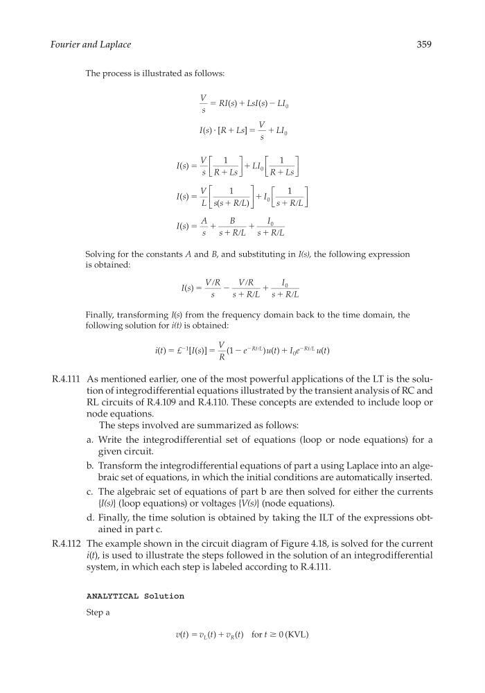
The process is illustrated as follows:
V
s
RI s LsI s LI
I s R Ls
V
s
LI
ϭ
ϩ
ϩ
ϭ ϩ
( )
( )
( ) [
]
Ϫ
и
0
0
I s
V
s R Ls
LI
R Ls
I s
V
L s s R L
I
( )
( )
(
)
ϭ
ϩ
ϩ
ϩ
ϭ
ϩ
ϩ
1
1
1
0
0
ր
1 1
0
s R L
I s
A
s
B
s R L
I
s R L
ϩ
ϭ ϩ ϩ
ϩ ϩ
ր
ր
ր
( )
Solving for the constants A and B, and substituting in I(s), the following expression
is obtained:
I s
V R
s
V R
s R L
I
s R L
( ) ϭ
ϩ
ϩ ϩ
ր Ϫ
ր
ր
ր
0
Finally, transforming I(s) from the frequency domain back to the time domain, the
following solution for i(t) is obtained:
i t
I s
V
R
e
ut
I e
ut
Rt L
Rt L
( )
[ ( )]
(
) ( )
( )
ϭ
ϭ
ϩ
£
Ϫ
Ϫ ր
Ϫ ր
Ϫ
1
0
1
R.4.111 As mentioned earlier, one of the most powerful applications of the LT is the solution of integrodifferential equations illustrated by the transient analysis of RC and
RL circuits of R.4.109 and R.4.110. These concepts are extended to include loop or
node equations.
The steps involved are summarized as follows:
a. Write the integrodifferential set of equations (loop or node equations) for a
given circuit.
b. Transform the integrodifferential equations of part a using Laplace into an algebraic set of equations, in which the initial conditions are automatically inserted.
c. The algebraic set of equations of part b are then solved for either the currents
{I(s)} (loop equations) or voltages {V(s)} (node equations).
d. Finally, the time solution is obtained by taking the ILT of the expressions obtained in part c.
R.4.112 The example shown in the circuit diagram of Figure 4.18, is solved for the current
i(t), is used to illustrate the steps followed in the solution of an integrodifferential
system, in which each step is labeled according to R.4.111.
ANALYTICAL Solution
Step a
v t
v t v t
t
L
R
( )
( )
( )
(
)
ϭ
ϩ
for
KVL
Ն 0
CRC_47760_CH004.indd 359
CRC_47760_CH004.indd 359
7/28/2008 12:26:02 PM
7/28/2008 12:26:02 PM
359
The process is illustrated as follows:
V
s
RI s LsI s LI
I s R Ls
V
s
LI
ϭ
ϩ
ϩ
ϭ ϩ
( )
( )
( ) [
]
Ϫ
и
0
0
I s
V
s R Ls
LI
R Ls
I s
V
L s s R L
I
( )
( )
(
)
ϭ
ϩ
ϩ
ϩ
ϭ
ϩ
ϩ
1
1
1
0
0
ր
1 1
0
s R L
I s
A
s
B
s R L
I
s R L
ϩ
ϭ ϩ ϩ
ϩ ϩ
ր
ր
ր
( )
Solving for the constants A and B, and substituting in I(s), the following expression
is obtained:
I s
V R
s
V R
s R L
I
s R L
( ) ϭ
ϩ
ϩ ϩ
ր Ϫ
ր
ր
ր
0
Finally, transforming I(s) from the frequency domain back to the time domain, the
following solution for i(t) is obtained:
i t
I s
V
R
e
ut
I e
ut
Rt L
Rt L
( )
[ ( )]
(
) ( )
( )
ϭ
ϭ
ϩ
£
Ϫ
Ϫ ր
Ϫ ր
Ϫ
1
0
1
R.4.111 As mentioned earlier, one of the most powerful applications of the LT is the solution of integrodifferential equations illustrated by the transient analysis of RC and
RL circuits of R.4.109 and R.4.110. These concepts are extended to include loop or
node equations.
The steps involved are summarized as follows:
a. Write the integrodifferential set of equations (loop or node equations) for a
given circuit.
b. Transform the integrodifferential equations of part a using Laplace into an algebraic set of equations, in which the initial conditions are automatically inserted.
c. The algebraic set of equations of part b are then solved for either the currents
{I(s)} (loop equations) or voltages {V(s)} (node equations).
d. Finally, the time solution is obtained by taking the ILT of the expressions obtained in part c.
R.4.112 The example shown in the circuit diagram of Figure 4.18, is solved for the current
i(t), is used to illustrate the steps followed in the solution of an integrodifferential
system, in which each step is labeled according to R.4.111.
ANALYTICAL Solution
Step a
v t
v t v t
t
L
R
( )
( )
( )
(
)
ϭ
ϩ
for
KVL
Ն 0
CRC_47760_CH004.indd 359
CRC_47760_CH004.indd 359
7/28/2008 12:26:02 PM
7/28/2008 12:26:02 PM