

358
Practical MATLAB
® Applications for Engineers
Then, applying Kirchhoff’s voltage law to the loop of the circuit diagram, shown in
Figure 4.15, and performing some algebraic manipulation the current I(s) can be solved,
and an expression for i(t) (ILT) can be obtained, as indicated in the following:
V
s
RI s
I s
sC
V
s
I s R
I s
sC
V
s
V
s
I s R
sC
V V
ϭ
ϩ
ϩ
ϩ
ϭ
ϩ
ϭ
( )
( )
( )
( )
( )
0
0
0
1
Ϫ
Ϫ
s s
I s
V V
R
s
R C
⋅
( )
(
)
ϭ
ϩ
Ϫ
ր
0
1
1
and the current i(t) is therefore given by
i t
I s
V V
R
e
u t
t RC
( )
( )
( )
ϭ
ϭ
£
Ϫ
Ϫ ր
Ϫ
1
0
[ ]
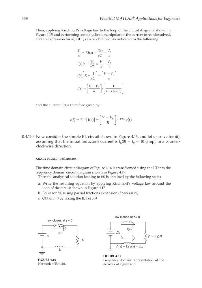
R.4.110 Now consider the simple RL circuit shown in Figure 4.16, and let us solve for i(t),
assuming that the initial inductor’s current is I L (0) = I 0 = 10 (amp), in a counterclockwise direction.
ANALYTICAL Solution
The time domain circuit diagram of Figure 4.16 is transformed using the LT into the
frequency domain circuit diagram shown in Figure 4.17.
Then the analytical solution leading to i(t) is obtained by the following steps:
a. Write the resulting equation by applying Kirchhoff’s voltage law around the
loop of the circuit shown in Figure 4.17
b. Solve for I(s) (using partial fractions expansion if necessary)
c. Obtain i(t) by taking the ILT of I(s)
V
R
sw closes at t = 0
i(t)
L
FIGURE 4.16
Network of R.4.110.
V/s
Vr = I(s)R
sw closes at t = 0
I(s)
Vl(s) = Ls I(s) − LI 0
I 0
FIGURE 4.17
Frequency domain representation of the
network of Figure 4.16.
CRC_47760_CH004.indd 358
CRC_47760_CH004.indd 358
7/28/2008 12:26:01 PM
7/28/2008 12:26:01 PM
Practical MATLAB
® Applications for Engineers
Then, applying Kirchhoff’s voltage law to the loop of the circuit diagram, shown in
Figure 4.15, and performing some algebraic manipulation the current I(s) can be solved,
and an expression for i(t) (ILT) can be obtained, as indicated in the following:
V
s
RI s
I s
sC
V
s
I s R
I s
sC
V
s
V
s
I s R
sC
V V
ϭ
ϩ
ϩ
ϩ
ϭ
ϩ
ϭ
( )
( )
( )
( )
( )
0
0
0
1
Ϫ
Ϫ
s s
I s
V V
R
s
R C
⋅
( )
(
)
ϭ
ϩ
Ϫ
ր
0
1
1
and the current i(t) is therefore given by
i t
I s
V V
R
e
u t
t RC
( )
( )
( )
ϭ
ϭ
£
Ϫ
Ϫ ր
Ϫ
1
0
[ ]
R.4.110 Now consider the simple RL circuit shown in Figure 4.16, and let us solve for i(t),
assuming that the initial inductor’s current is I L (0) = I 0 = 10 (amp), in a counterclockwise direction.
ANALYTICAL Solution
The time domain circuit diagram of Figure 4.16 is transformed using the LT into the
frequency domain circuit diagram shown in Figure 4.17.
Then the analytical solution leading to i(t) is obtained by the following steps:
a. Write the resulting equation by applying Kirchhoff’s voltage law around the
loop of the circuit shown in Figure 4.17
b. Solve for I(s) (using partial fractions expansion if necessary)
c. Obtain i(t) by taking the ILT of I(s)
V
R
sw closes at t = 0
i(t)
L
FIGURE 4.16
Network of R.4.110.
V/s
Vr = I(s)R
sw closes at t = 0
I(s)
Vl(s) = Ls I(s) − LI 0
I 0
FIGURE 4.17
Frequency domain representation of the
network of Figure 4.16.
CRC_47760_CH004.indd 358
CRC_47760_CH004.indd 358
7/28/2008 12:26:01 PM
7/28/2008 12:26:01 PM