

354
Practical MATLAB
® Applications for Engineers
where y(t) = £
−1 [Y(s)]. The process of evaluating the coeffi cients A, B, and C by hand
is illustrated as follows:
A
s
s
s s
s
s
ϭ
ϩ
ϩ
ϭ
ϭ
ϭ
(
) ()
(
)(
)
( )( )
4
10
1
2
10
1 2
5
0
⋅
Ϫ
Ϫ Ϫ
B
s
s
s s
s
s
ϭ
ϩ
ϩ
ϩ
ϩ
ϭ
ϭ
(
) (
)
(
)(
)
4
10
1
1
2
6
1
Ϫ
Ϫ
C
s
s
s s
s
s
ϭ
ϩ
ϩ
ϩ
ϩ
ϭ
ϭ
(
) (
)
(
)(
)
4
10
2
1
2
1
2
Ϫ
then
Y s
s s
s
( ) ϭ
ϩ
ϩ ϩ
5
6
1
1
2
Ϫ
and
y(t) = £
−1 [Y(s)] = 5u(t) − 6e
−t u(t) + e
−2t u(t)
R.4.99 Let us use the concepts developed by the Laplace technique, in the analysis of electrical networks. Recall that v R (t) = R i(t) (Ohm’s law), and its Laplace transform is
given by £ [v R (t)] = £[R ⋅ i(t)] = R £[i(t)], then
V R (s) = R * I(s)
Ohm’s law holds in the frequency domain, and the impedance Z(s) (Ω) is defi ned by
Z s
V s
I s
( )
( )
( )
ϭ
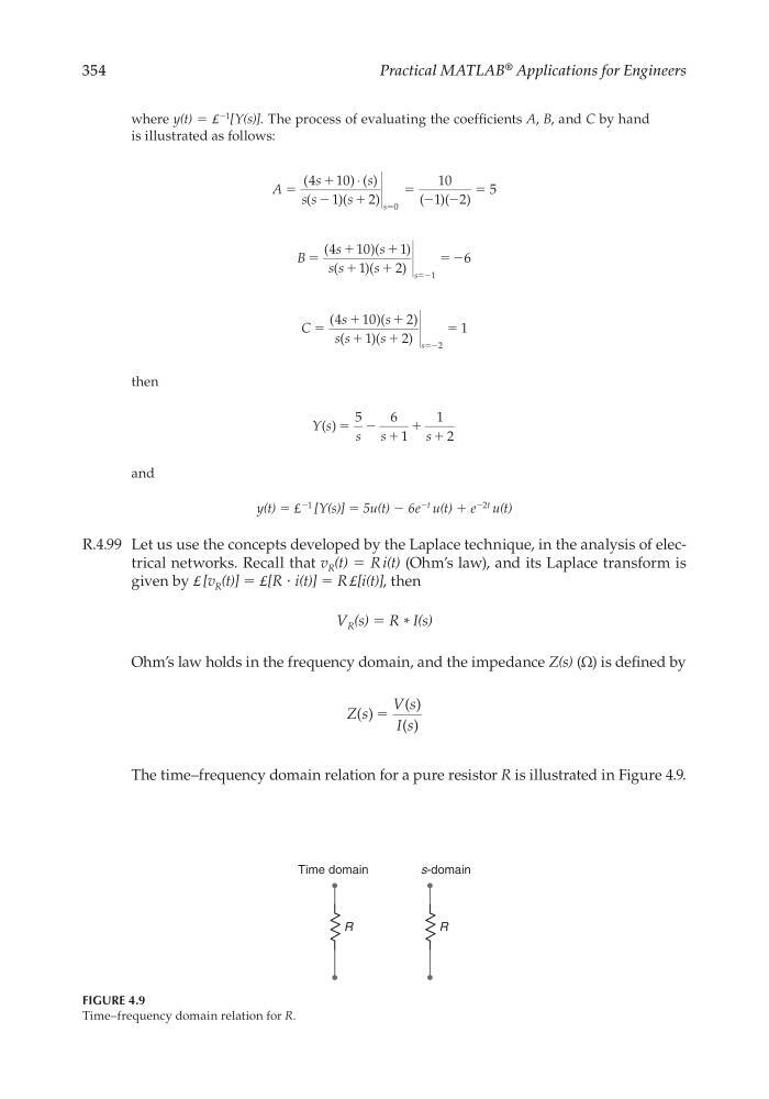
The time–frequency domain relation for a pure resistor R is illustrated in Figure 4.9.
R
R
Time domain
s-domain
FIGURE 4.9
Time–frequency domain relation for R.
CRC_47760_CH004.indd 354
CRC_47760_CH004.indd 354
7/28/2008 12:25:59 PM
7/28/2008 12:25:59 PM
Practical MATLAB
® Applications for Engineers
where y(t) = £
−1 [Y(s)]. The process of evaluating the coeffi cients A, B, and C by hand
is illustrated as follows:
A
s
s
s s
s
s
ϭ
ϩ
ϩ
ϭ
ϭ
ϭ
(
) ()
(
)(
)
( )( )
4
10
1
2
10
1 2
5
0
⋅
Ϫ
Ϫ Ϫ
B
s
s
s s
s
s
ϭ
ϩ
ϩ
ϩ
ϩ
ϭ
ϭ
(
) (
)
(
)(
)
4
10
1
1
2
6
1
Ϫ
Ϫ
C
s
s
s s
s
s
ϭ
ϩ
ϩ
ϩ
ϩ
ϭ
ϭ
(
) (
)
(
)(
)
4
10
2
1
2
1
2
Ϫ
then
Y s
s s
s
( ) ϭ
ϩ
ϩ ϩ
5
6
1
1
2
Ϫ
and
y(t) = £
−1 [Y(s)] = 5u(t) − 6e
−t u(t) + e
−2t u(t)
R.4.99 Let us use the concepts developed by the Laplace technique, in the analysis of electrical networks. Recall that v R (t) = R i(t) (Ohm’s law), and its Laplace transform is
given by £ [v R (t)] = £[R ⋅ i(t)] = R £[i(t)], then
V R (s) = R * I(s)
Ohm’s law holds in the frequency domain, and the impedance Z(s) (Ω) is defi ned by
Z s
V s
I s
( )
( )
( )
ϭ
The time–frequency domain relation for a pure resistor R is illustrated in Figure 4.9.
R
R
Time domain
s-domain
FIGURE 4.9
Time–frequency domain relation for R.
CRC_47760_CH004.indd 354
CRC_47760_CH004.indd 354
7/28/2008 12:25:59 PM
7/28/2008 12:25:59 PM