

Fourier and Laplace
351
poles =
-1.0000 + 1.0000i
-1.0000 - 1.0000i
-1.0000
**************************************************
The ROC lie in the region given by: real part greater than
real _ s =
-1.0000
**************************************************
Region of convergence
Pole−zero map
1.5
0.5
0
−0.5
−1
−1.5
−3
−2.5
−2
−1.5
−1
−0.5
0
0.5
1
1.5
2
1
Real axis
Imaginary axis
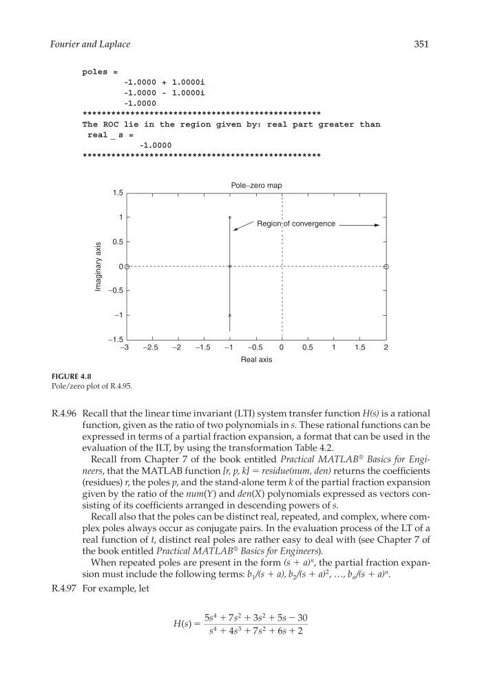
FIGURE 4.8
Pole/zero plot of R.4.95.
R.4.96 Recall that the linear time invariant (LTI) system transfer function H(s) is a rational
function, given as the ratio of two polynomials in s. These rational functions can be
expressed in terms of a partial fraction expansion, a format that can be used in the
evaluation of the ILT, by using the transformation Table 4.2.
Recall from Chapter 7 of the book entitled Practical MATLAB
® Basics for Engineers, that the MATLAB function [r, p, k] = residue(num, den) returns the coeffi cients
(residues) r, the poles p, and the stand-alone term k of the partial fraction expansion
given by the ratio of the num(Y) and den(X) polynomials expressed as vectors consisting of its coeffi cients arranged in descending powers of s.
Recall also that the poles can be distinct real, repeated, and complex, where complex poles always occur as conjugate pairs. In the evaluation process of the LT of a
real function of t, distinct real poles are rather easy to deal with (see Chapter 7 of
the book entitled Practical MATLAB
® Basics for Engineers).
When repeated poles are present in the form (s + a)
n
, the partial fraction expansion must include the following terms: b 1 /(s + a), b 2 /(s + a)
2 , …, b n /(s + a)
n .
R.4.97 For example, let
H s
s
s
s
s
s
s
s
s
( ) ϭ
ϩ
ϩ
ϩ Ϫ
ϩ
ϩ
ϩ ϩ
5
7
3
5
30
4
7
6
2
4
2
2
4
3
2
CRC_47760_CH004.indd 351
CRC_47760_CH004.indd 351
7/28/2008 12:25:58 PM
7/28/2008 12:25:58 PM
351
poles =
-1.0000 + 1.0000i
-1.0000 - 1.0000i
-1.0000
**************************************************
The ROC lie in the region given by: real part greater than
real _ s =
-1.0000
**************************************************
Region of convergence
Pole−zero map
1.5
0.5
0
−0.5
−1
−1.5
−3
−2.5
−2
−1.5
−1
−0.5
0
0.5
1
1.5
2
1
Real axis
Imaginary axis
FIGURE 4.8
Pole/zero plot of R.4.95.
R.4.96 Recall that the linear time invariant (LTI) system transfer function H(s) is a rational
function, given as the ratio of two polynomials in s. These rational functions can be
expressed in terms of a partial fraction expansion, a format that can be used in the
evaluation of the ILT, by using the transformation Table 4.2.
Recall from Chapter 7 of the book entitled Practical MATLAB
® Basics for Engineers, that the MATLAB function [r, p, k] = residue(num, den) returns the coeffi cients
(residues) r, the poles p, and the stand-alone term k of the partial fraction expansion
given by the ratio of the num(Y) and den(X) polynomials expressed as vectors consisting of its coeffi cients arranged in descending powers of s.
Recall also that the poles can be distinct real, repeated, and complex, where complex poles always occur as conjugate pairs. In the evaluation process of the LT of a
real function of t, distinct real poles are rather easy to deal with (see Chapter 7 of
the book entitled Practical MATLAB
® Basics for Engineers).
When repeated poles are present in the form (s + a)
n
, the partial fraction expansion must include the following terms: b 1 /(s + a), b 2 /(s + a)
2 , …, b n /(s + a)
n .
R.4.97 For example, let
H s
s
s
s
s
s
s
s
s
( ) ϭ
ϩ
ϩ
ϩ Ϫ
ϩ
ϩ
ϩ ϩ
5
7
3
5
30
4
7
6
2
4
2
2
4
3
2
CRC_47760_CH004.indd 351
CRC_47760_CH004.indd 351
7/28/2008 12:25:58 PM
7/28/2008 12:25:58 PM