Alternating Current Analysis
297
Example 3.17
The objective of this example is to verify the maximum power transfer theorem, when
the load resistance varies over a given range.
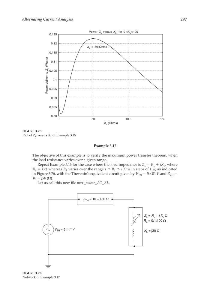
Repeat Example 3.16 for the case where the load impedance is Z L = R L + jX L , where
X L = j30, whereas R L varies over the range 1 ≤ R L ≤ 100 Ω in steps of 1 Ω, as indicated
in Figure 3.76, with the Thevenin’s equivalent circuit given by V TH = 5 ∠0° V and Z TH =
10 − j50 (Ω).
Let us call this new fi le max_power_AC_RL.
0
50
100
150
0.08
0.085
0.09
0.095
0.1
0.105
0.11
0.115
0.12
0.125
X L (Ohms)
Power deliver to Z
L (Watts)
Power Z L versus X L , for 0 X L = 50j Ohms
FIGURE 3.75
Plot of Z L versus X L of Example 3.16.
Z TH = 10 − j 50 Ω
Z L = R L + j X L Ω
V TH = 5 0° V
R L = 0:1:100 Ω
X L = j30 Ω
FIGURE 3.76
Network of Example 3.17.
CRC_47760_CH003.indd 297
CRC_47760_CH003.indd 297
7/23/2008 1:27:51 PM
7/23/2008 1:27:51 PM