296
Practical MATLAB
® Applications for Engineers
Example 3.16
The objective of this example is to verify the maximum power transfer theorem, when
the load reactance varies over a given range.
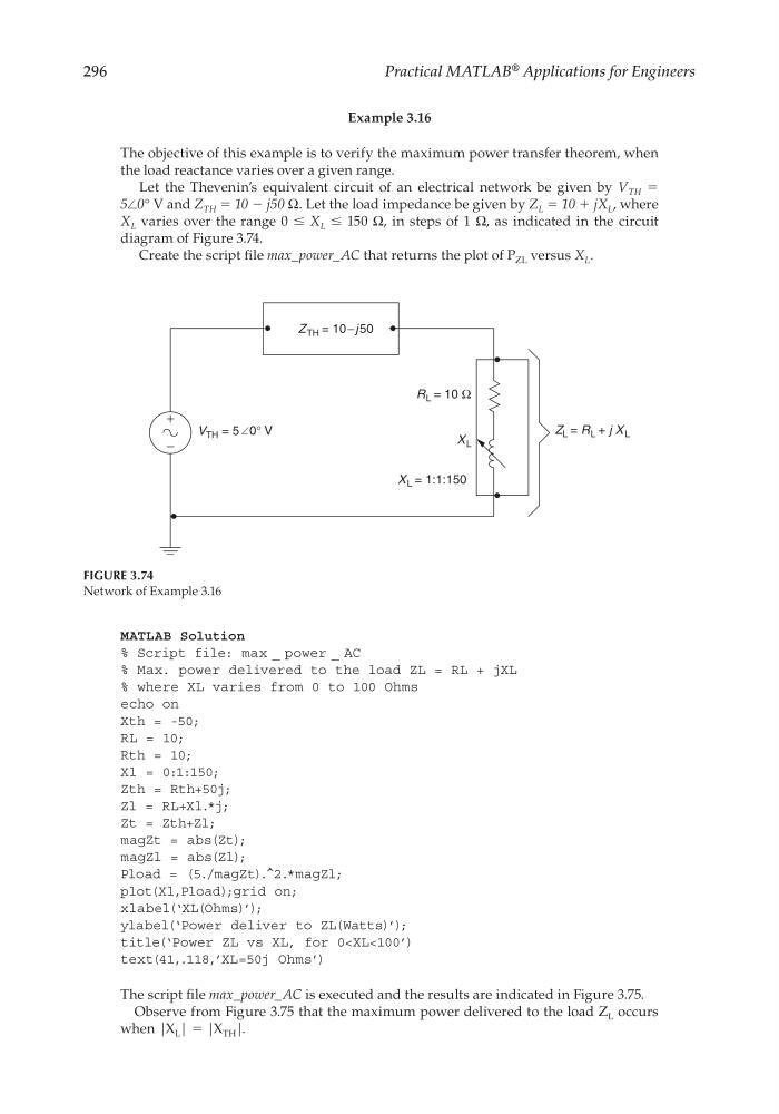
Let the Thevenin’s equivalent circuit of an electrical network be given by V TH =
5∠0° V and Z TH = 10 − j50 Ω. Let the load impedance be given by Z L = 10 + jX L , where
X L varies over the range 0 ≤ X L ≤ 150 Ω, in steps of 1 Ω, as indicated in the circuit
diagram of Figure 3.74.
Create the script fi le max_power_AC that returns the plot of P ZL versus X L .
X L
X L = 1:1:150
R L = 10 Ω
Z TH = 10 − j 50
V TH = 5 0° V
Z L = R L + j X L
FIGURE 3.74
Network of Example 3.16
MATLAB Solution
% Script file: max _ power _ AC
% Max. power delivered to the load ZL = RL + jXL
% where XL varies from 0 to 100 Ohms
echo on
Xth = -50;
RL = 10;
Rth = 10;
Xl = 0:1:150;
Zth = Rth+50j;
Zl = RL+Xl.*j;
Zt = Zth+Zl;
magZt = abs(Zt);
magZl = abs(Zl);
Pload = (5./magZt).^2.*magZl;
plot(Xl,Pload);grid on;
xlabel(‘XL(Ohms)’);
ylabel(‘Power deliver to ZL(Watts)’);
title(‘Power ZL vs XL, for 0 text(41,.118,’XL=50j Ohms’)
The script fi le max_power_AC is executed and the results are indicated in Figure 3.75.
Observe from Figure 3.75 that the maximum power delivered to the load Z L occurs
when |X L | = |X TH |.
CRC_47760_CH003.indd 296
CRC_47760_CH003.indd 296
7/23/2008 1:27:51 PM
7/23/2008 1:27:51 PM