

256
Practical MATLAB
® Applications for Engineers
Then,
Z TH = [(Z 1 | |Z 2 ) + Z 3 ] | |Z 4 Ω
Z | |Z Z
j
j
j
j
1
2
3
ϩ ϭ
ϩ
Ϫ
ϩ ϩ ϭ
ϩ
(
)(
)
.
.
6
2 4
2
10
6
2 8 8
1 6 Ω
and
Z
j
j
j
j
TH ϭ
ϩ
ϩ
ϩ
ϭ
ϩ
( .
. ) * (
)
.
.
8 8
1 6
11
2
19 8
3 6
44
9
8
9
Ω
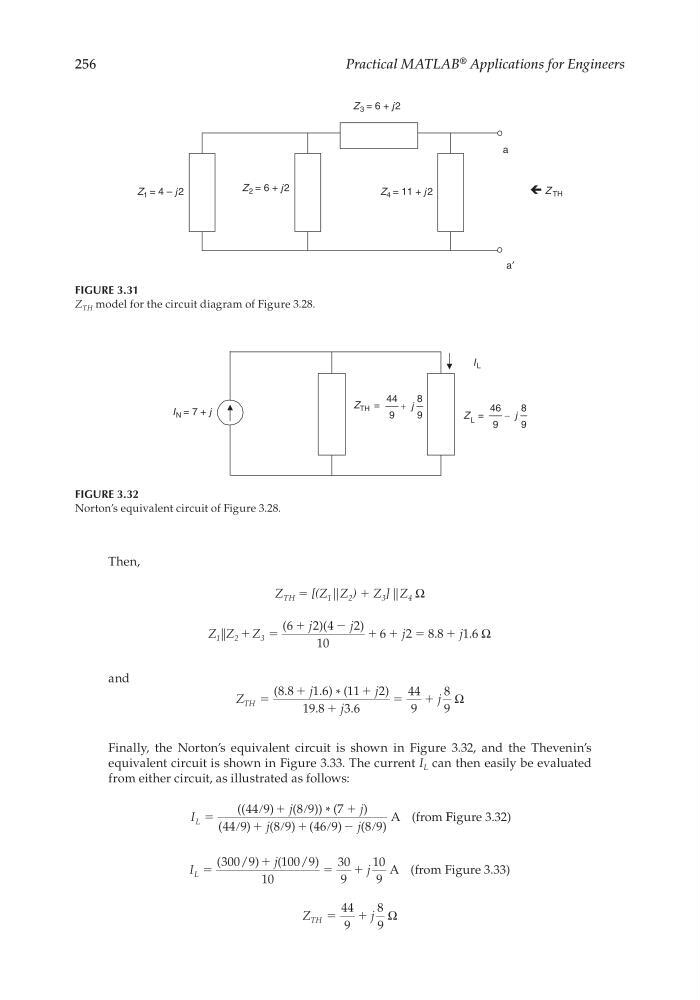
Finally, the Norton’s equivalent circuit is shown in Figure 3.32, and the Thevenin’s
equivalent circuit is shown in Figure 3.33. The current I L can then easily be evaluated
from either circuit, as illustrated as follows:
I
j
j
j
j
L ϭ
ր ϩ ր
ϩ
ր ϩ ր ϩ
ր Ϫ ր
((
) ( )) * (
)
(
) ( ) (
)
( )
44 9
8 9
7
44 9
8 9
46 9
8 9
A (from F Figure 3.32)
I
j
j
L ϭ
ϩ
ϭ
ϩ
(
/ ) (
/ )
300 9
100 9
10
30
9
10
9
A (from Figure 3.33)
Z
j
TH ϭ
ϩ
44
9
8
9
Ω
a′
Z 1 = 4 – j 2
Z 4 = 11 + j 2
Z 2 = 6 + j2
Z TH
a
Z 3 = 6 + j 2
FIGURE 3.31
Z TH model for the circuit diagram of Figure 3.28.
I N = 7 + j
Z L =
9
8
9
46
j
−
Z TH =
9
8
9
44
j
+
I L
FIGURE 3.32
Norton’s equivalent circuit of Figure 3.28.
CRC_47760_CH003.indd 256
CRC_47760_CH003.indd 256
7/23/2008 1:27:39 PM
7/23/2008 1:27:39 PM
Practical MATLAB
® Applications for Engineers
Then,
Z TH = [(Z 1 | |Z 2 ) + Z 3 ] | |Z 4 Ω
Z | |Z Z
j
j
j
j
1
2
3
ϩ ϭ
ϩ
Ϫ
ϩ ϩ ϭ
ϩ
(
)(
)
.
.
6
2 4
2
10
6
2 8 8
1 6 Ω
and
Z
j
j
j
j
TH ϭ
ϩ
ϩ
ϩ
ϭ
ϩ
( .
. ) * (
)
.
.
8 8
1 6
11
2
19 8
3 6
44
9
8
9
Ω
Finally, the Norton’s equivalent circuit is shown in Figure 3.32, and the Thevenin’s
equivalent circuit is shown in Figure 3.33. The current I L can then easily be evaluated
from either circuit, as illustrated as follows:
I
j
j
j
j
L ϭ
ր ϩ ր
ϩ
ր ϩ ր ϩ
ր Ϫ ր
((
) ( )) * (
)
(
) ( ) (
)
( )
44 9
8 9
7
44 9
8 9
46 9
8 9
A (from F Figure 3.32)
I
j
j
L ϭ
ϩ
ϭ
ϩ
(
/ ) (
/ )
300 9
100 9
10
30
9
10
9
A (from Figure 3.33)
Z
j
TH ϭ
ϩ
44
9
8
9
Ω
a′
Z 1 = 4 – j 2
Z 4 = 11 + j 2
Z 2 = 6 + j2
Z TH
a
Z 3 = 6 + j 2
FIGURE 3.31
Z TH model for the circuit diagram of Figure 3.28.
I N = 7 + j
Z L =
9
8
9
46
j
−
Z TH =
9
8
9
44
j
+
I L
FIGURE 3.32
Norton’s equivalent circuit of Figure 3.28.
CRC_47760_CH003.indd 256
CRC_47760_CH003.indd 256
7/23/2008 1:27:39 PM
7/23/2008 1:27:39 PM