

234
Practical MATLAB
® Applications for Engineers
R.3.29 Let us assume that the voltage across the capacitor C is v C (t) = V m cos(ωt) in volts,
then its current is given by
i t
C
dv t
dt
C
d
dt
V
t
C
c
m
( )
( )
[ cos( )]
ϭ
ϭ
i t
C V
t
CV
t
C
m
m
( )
sin( )
cos
ϭ Ϫ
ϭ
ϩ
2
Let
i t
I
t
C
m
( )
cos
ϭ
ϩ
2
then
I
CV
m
m
ϭ
or by Ohm’s law
X
j C
j
C ( )
ϭ
Ϫ
1
2
where denotes a phase angle of
R.3.30 Let the voltage across C be v C (t) = V m cos(ωt) (from R.3.29), then the current through
C is given by i C (t) = I m cos(ωt + (π/2)). Clearly, the current leads the voltage by an
angle of π/2 rad. Capacitive reactance X C represents the opposition to the fl ow of
charge, which results in the continuous interchange of energy between the source
and the electric fi eld of the capacitor.
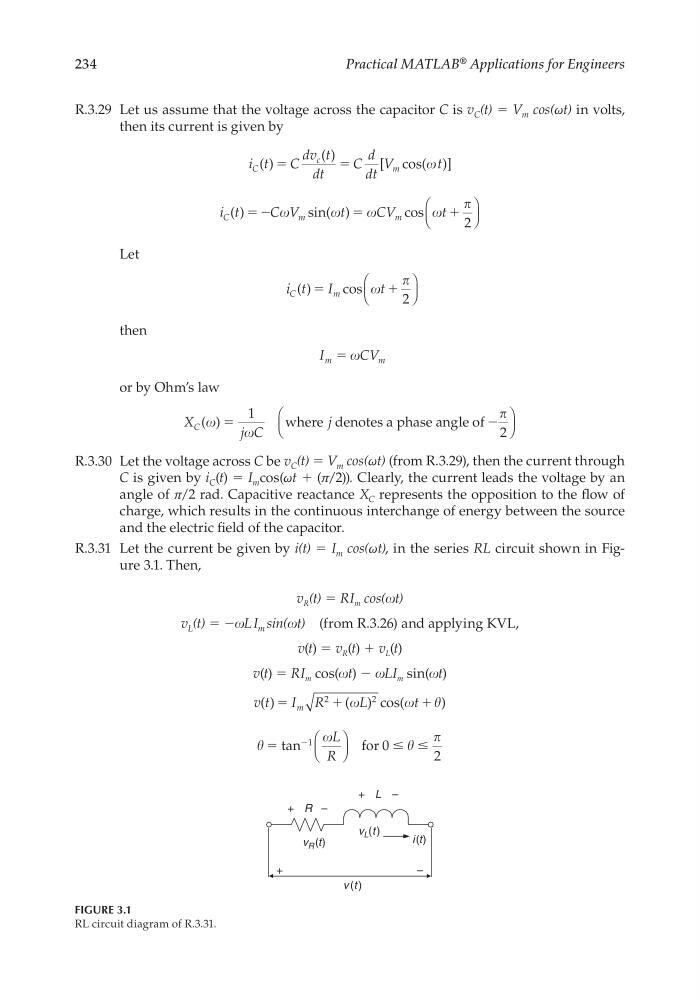
R.3.31 Let the current be given by i(t) = I m cos(ωt), in the series RL circuit shown in Figure 3.1. Then,
v R (t) = RI m cos(t)
v L (t) = −L I m sin(t) (from R.3.26) and applying KVL,
v (t) = v R (t) + v L (t)
v (t) = RI m cos(t) − LI m sin(t)
v t
I R
L
t
m
( )
( ) cos(
)
ϭ
ϩ
ϩ
2
2
ϭ
Յ Յ
Ϫ
tan
1
0
2
L
R
for
FIGURE 3.1
RL circuit diagram of R.3.31.
+ L –
+ R –
v R (t)
i (t)
v (t )
v L (t )
–
+
CRC_47760_CH003.indd 234
CRC_47760_CH003.indd 234
7/23/2008 1:27:31 PM
7/23/2008 1:27:31 PM
Practical MATLAB
® Applications for Engineers
R.3.29 Let us assume that the voltage across the capacitor C is v C (t) = V m cos(ωt) in volts,
then its current is given by
i t
C
dv t
dt
C
d
dt
V
t
C
c
m
( )
( )
[ cos( )]
ϭ
ϭ
i t
C V
t
CV
t
C
m
m
( )
sin( )
cos
ϭ Ϫ
ϭ
ϩ
2
Let
i t
I
t
C
m
( )
cos
ϭ
ϩ
2
then
I
CV
m
m
ϭ
or by Ohm’s law
X
j C
j
C ( )
ϭ
Ϫ
1
2
where denotes a phase angle of
R.3.30 Let the voltage across C be v C (t) = V m cos(ωt) (from R.3.29), then the current through
C is given by i C (t) = I m cos(ωt + (π/2)). Clearly, the current leads the voltage by an
angle of π/2 rad. Capacitive reactance X C represents the opposition to the fl ow of
charge, which results in the continuous interchange of energy between the source
and the electric fi eld of the capacitor.
R.3.31 Let the current be given by i(t) = I m cos(ωt), in the series RL circuit shown in Figure 3.1. Then,
v R (t) = RI m cos(t)
v L (t) = −L I m sin(t) (from R.3.26) and applying KVL,
v (t) = v R (t) + v L (t)
v (t) = RI m cos(t) − LI m sin(t)
v t
I R
L
t
m
( )
( ) cos(
)
ϭ
ϩ
ϩ
2
2
ϭ
Յ Յ
Ϫ
tan
1
0
2
L
R
for
FIGURE 3.1
RL circuit diagram of R.3.31.
+ L –
+ R –
v R (t)
i (t)
v (t )
v L (t )
–
+
CRC_47760_CH003.indd 234
CRC_47760_CH003.indd 234
7/23/2008 1:27:31 PM
7/23/2008 1:27:31 PM