

190
Practical MATLAB
® Applications for Engineers
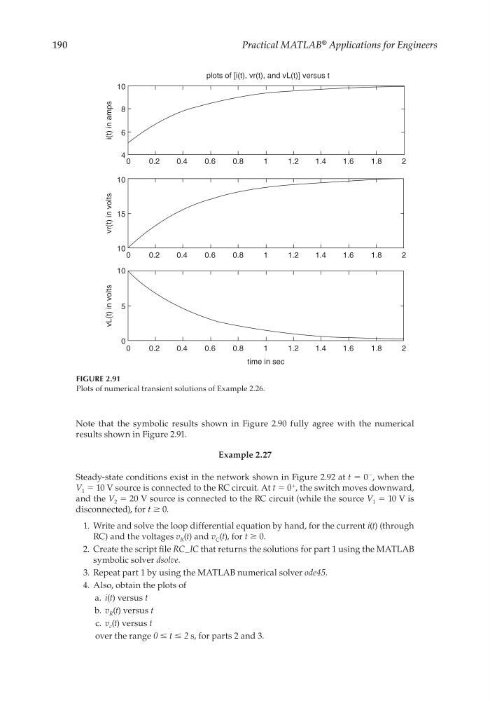
Note that the symbolic results shown in Figure 2.90 fully agree with the numerical
results shown in Figure 2.91.
Example 2.27
Steady-state conditions exist in the network shown in Figure 2.92 at t = 0
−
, when the
V 1 = 10 V source is connected to the RC circuit. At t = 0
+
, the switch moves downward,
and the V 2 = 20 V source is connected to the RC circuit (while the source V 1 = 10 V is
disconnected), for t ≥ 0.
1. Write and solve the loop differential equation by hand, for the current i(t) (through
RC) and the voltages v R (t) and v C (t), for t ≥ 0.
2. Create the script fi le RC_IC that returns the solutions for part 1 using the MATLAB
symbolic solver dsolve.
3. Repeat part 1 by using the MATLAB numerical solver ode45.
4. Also, obtain the plots of
a. i(t) versus t
b. v R (t) versus t
c. v c (t) versus t
over the range 0 ≤ t ≤ 2 s, for parts 2 and 3.
FIGURE 2.91
Plots of numerical transient solutions of Example 2.26.
2
1.8
1.6
1.4
1.2
1
0.8
0.6
0.4
0.2
0
6
4
8
10
plots of [i(t), vr(t), and vL(t)] versus t
i(t) in amps
vr(t) in volts
vL(t) in volts
2
1.8
1.6
1.4
1.2
1
0.8
0.6
0.4
0.2
0
10
15
10
2
1.8
1.6
1.4
1.2
1
0.8
time in sec
0.6
0.4
0.2
0
0
5
10
CRC_47760_CH002.indd 190
CRC_47760_CH002.indd 190
7/23/2008 1:38:58 PM
7/23/2008 1:38:58 PM
Practical MATLAB
® Applications for Engineers
Note that the symbolic results shown in Figure 2.90 fully agree with the numerical
results shown in Figure 2.91.
Example 2.27
Steady-state conditions exist in the network shown in Figure 2.92 at t = 0
−
, when the
V 1 = 10 V source is connected to the RC circuit. At t = 0
+
, the switch moves downward,
and the V 2 = 20 V source is connected to the RC circuit (while the source V 1 = 10 V is
disconnected), for t ≥ 0.
1. Write and solve the loop differential equation by hand, for the current i(t) (through
RC) and the voltages v R (t) and v C (t), for t ≥ 0.
2. Create the script fi le RC_IC that returns the solutions for part 1 using the MATLAB
symbolic solver dsolve.
3. Repeat part 1 by using the MATLAB numerical solver ode45.
4. Also, obtain the plots of
a. i(t) versus t
b. v R (t) versus t
c. v c (t) versus t
over the range 0 ≤ t ≤ 2 s, for parts 2 and 3.
FIGURE 2.91
Plots of numerical transient solutions of Example 2.26.
2
1.8
1.6
1.4
1.2
1
0.8
0.6
0.4
0.2
0
6
4
8
10
plots of [i(t), vr(t), and vL(t)] versus t
i(t) in amps
vr(t) in volts
vL(t) in volts
2
1.8
1.6
1.4
1.2
1
0.8
0.6
0.4
0.2
0
10
15
10
2
1.8
1.6
1.4
1.2
1
0.8
time in sec
0.6
0.4
0.2
0
0
5
10
CRC_47760_CH002.indd 190
CRC_47760_CH002.indd 190
7/23/2008 1:38:58 PM
7/23/2008 1:38:58 PM