

152
Practical MATLAB
® Applications for Engineers
ANALYTICAL Solution
Recall that
R
L
A
T
ϭ
ϩ
(1 TC *
)
∆
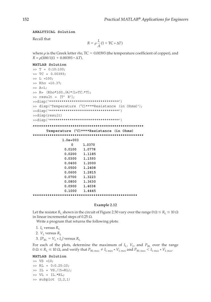
where ρ is the Greek letter rho, TC = 0.00393 (the temperature coeffi cient of copper), and
R = ρ(100/1)(1 + 0.00393 * ∆T).
MATLAB Solution
>> T = 0:10:100;
>> TC = 0.00393;
>> L =100;
>> Rho =10.37;
>> A=1;
>> R= (Rho*100./A)*(1+TC.*T);
>> result = [T’ R’];
>>disp(‘**********************************’)
>> disp(‘Temperature (°C)****Resistance (in Ohms)’);
>>disp(‘**********************************’)
>>disp(result)
>>disp(‘**********************************’)
*****************************************************
Temperature (°C)****Resistance (in Ohms)
*****************************************************
1.0e+003
0
1.0370
0.0100
1.0778
0.0200
1.1185
0.0300
1.1593
0.0400
1.2000
0.0500
1.2408
0.0600
1.2815
0.0700
1.3223
0.0800
1.3630
0.0900
1.4038
0.1000
1.4445
**************************************************
Example 2.12
Let the resistor R L shown in the circuit of Figure 2.50 vary over the range 0 Ω ≤ R L ≤ 10 Ω
in linear incremental steps of 0.25 Ω.
Write a program that returns the following plots:
1. I L versus R L
2. V L versus R L
3. [P RL = V L * I L ] versus R L
For each of the plots, determine the maximum of I L , V 2 , and P RL over the range
0 Ω ≤ R L ≤ 10 Ω, and verify that P RL-max ≠ I L-max * V L-max and P RL-max < I L-max * V L-max .
MATLAB Solution
>> VS =10;
>> RL = 0:0.25:10;
>> IL = VS./(5+RL);
>> VL = IL.*RL;
>> subplot (2,2,1)
CRC_47760_CH002.indd 152
CRC_47760_CH002.indd 152
7/23/2008 1:38:48 PM
7/23/2008 1:38:48 PM
Practical MATLAB
® Applications for Engineers
ANALYTICAL Solution
Recall that
R
L
A
T
ϭ
ϩ
(1 TC *
)
∆
where ρ is the Greek letter rho, TC = 0.00393 (the temperature coeffi cient of copper), and
R = ρ(100/1)(1 + 0.00393 * ∆T).
MATLAB Solution
>> T = 0:10:100;
>> TC = 0.00393;
>> L =100;
>> Rho =10.37;
>> A=1;
>> R= (Rho*100./A)*(1+TC.*T);
>> result = [T’ R’];
>>disp(‘**********************************’)
>> disp(‘Temperature (°C)****Resistance (in Ohms)’);
>>disp(‘**********************************’)
>>disp(result)
>>disp(‘**********************************’)
*****************************************************
Temperature (°C)****Resistance (in Ohms)
*****************************************************
1.0e+003
0
1.0370
0.0100
1.0778
0.0200
1.1185
0.0300
1.1593
0.0400
1.2000
0.0500
1.2408
0.0600
1.2815
0.0700
1.3223
0.0800
1.3630
0.0900
1.4038
0.1000
1.4445
**************************************************
Example 2.12
Let the resistor R L shown in the circuit of Figure 2.50 vary over the range 0 Ω ≤ R L ≤ 10 Ω
in linear incremental steps of 0.25 Ω.
Write a program that returns the following plots:
1. I L versus R L
2. V L versus R L
3. [P RL = V L * I L ] versus R L
For each of the plots, determine the maximum of I L , V 2 , and P RL over the range
0 Ω ≤ R L ≤ 10 Ω, and verify that P RL-max ≠ I L-max * V L-max and P RL-max < I L-max * V L-max .
MATLAB Solution
>> VS =10;
>> RL = 0:0.25:10;
>> IL = VS./(5+RL);
>> VL = IL.*RL;
>> subplot (2,2,1)
CRC_47760_CH002.indd 152
CRC_47760_CH002.indd 152
7/23/2008 1:38:48 PM
7/23/2008 1:38:48 PM