

Direct Current and Transient Analysis
149
>> plot (R2,I*1.0e3)
% current in ma
>> title (‘Current I, Voltage V2, and Voltage V1 vs R2’);
>> ylabel (‘Current I (mA)’)
>> grid on; V2 = R2.*I;
>> subplot(3,1,2)
>> plot (R2,V2)
>> ylabel (‘Voltage V2 (Volts)’)
>> grid on
>> subplot (3,1,3)
>> V1 = R1*I; plot(R2,V1)
>> xlabel (‘Resistance R2(Ohms)’),
>> ylabel (‘voltage V1(Volts)’)
>> grid on;
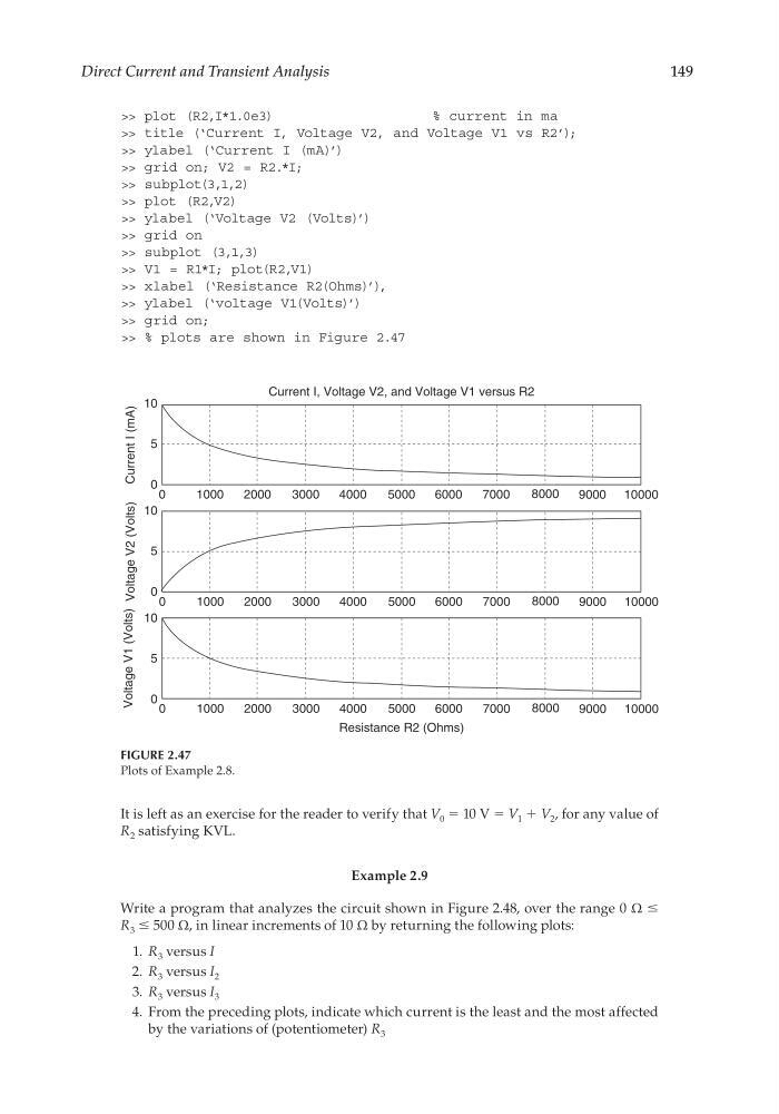
>> % plots are shown in Figure 2.47
FIGURE 2.47
Plots of Example 2.8.
0
1000
2000
3000
4000
5000
6000
7000
8000
9000 10000
0
1000
2000
3000
4000
5000
6000
7000
8000
9000 10000
0
0
5
10
0
5
10
0
5
Current I (mA)
Voltage V2 (Volts)
Voltage V1 (Volts)
10
1000
2000
3000
4000
5000
6000
Resistance R2 (Ohms)
7000
8000
9000 10000
Current I, Voltage V2, and Voltage V1 versus R2
It is left as an exercise for the reader to verify that V 0 = 10 V = V 1 + V 2 , for any value of
R 2 satisfying KVL.
Example 2.9
Write a program that analyzes the circuit shown in Figure 2.48, over the range 0 Ω ≤
R 3 ≤ 500 Ω, in linear increments of 10 Ω by returning the following plots:
1. R 3 versus I
2. R 3 versus I 2
3. R 3 versus I 3
4. From the preceding plots, indicate which current is the least and the most affected
by the variations of (potentiometer) R 3
CRC_47760_CH002.indd 149
CRC_47760_CH002.indd 149
7/23/2008 1:38:47 PM
7/23/2008 1:38:47 PM
149
>> plot (R2,I*1.0e3)
% current in ma
>> title (‘Current I, Voltage V2, and Voltage V1 vs R2’);
>> ylabel (‘Current I (mA)’)
>> grid on; V2 = R2.*I;
>> subplot(3,1,2)
>> plot (R2,V2)
>> ylabel (‘Voltage V2 (Volts)’)
>> grid on
>> subplot (3,1,3)
>> V1 = R1*I; plot(R2,V1)
>> xlabel (‘Resistance R2(Ohms)’),
>> ylabel (‘voltage V1(Volts)’)
>> grid on;
>> % plots are shown in Figure 2.47
FIGURE 2.47
Plots of Example 2.8.
0
1000
2000
3000
4000
5000
6000
7000
8000
9000 10000
0
1000
2000
3000
4000
5000
6000
7000
8000
9000 10000
0
0
5
10
0
5
10
0
5
Current I (mA)
Voltage V2 (Volts)
Voltage V1 (Volts)
10
1000
2000
3000
4000
5000
6000
Resistance R2 (Ohms)
7000
8000
9000 10000
Current I, Voltage V2, and Voltage V1 versus R2
It is left as an exercise for the reader to verify that V 0 = 10 V = V 1 + V 2 , for any value of
R 2 satisfying KVL.
Example 2.9
Write a program that analyzes the circuit shown in Figure 2.48, over the range 0 Ω ≤
R 3 ≤ 500 Ω, in linear increments of 10 Ω by returning the following plots:
1. R 3 versus I
2. R 3 versus I 2
3. R 3 versus I 3
4. From the preceding plots, indicate which current is the least and the most affected
by the variations of (potentiometer) R 3
CRC_47760_CH002.indd 149
CRC_47760_CH002.indd 149
7/23/2008 1:38:47 PM
7/23/2008 1:38:47 PM