

134
Practical MATLAB
® Applications for Engineers
where
w
w
d
o
ϭ
2
2
Ϫ
where A 1 and A 2 are constants that can be evaluated from the initial network
conditions.
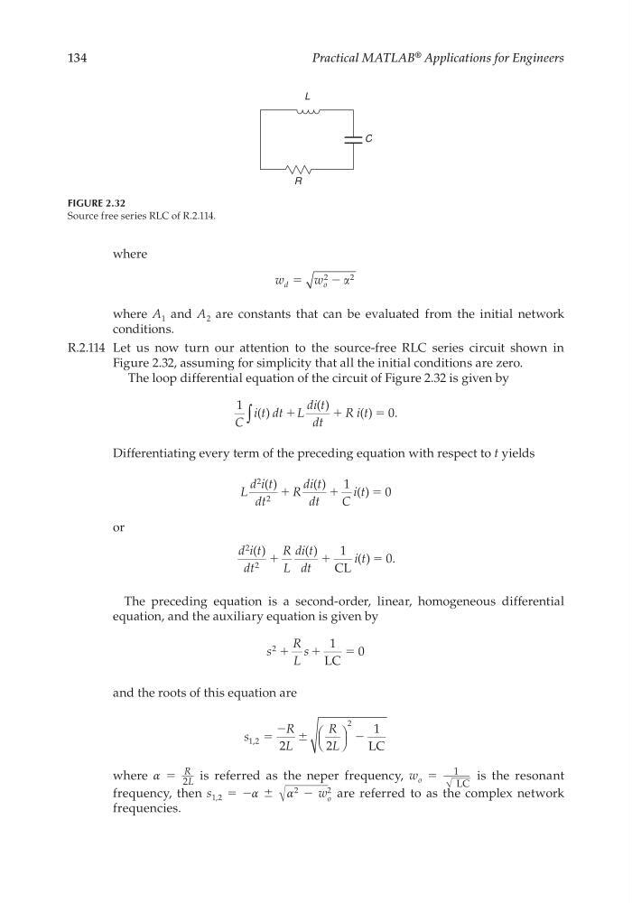
R.2.114 Let us now turn our attention to the source-free RLC series circuit shown in
Figure 2.32, assuming for simplicity that all the initial conditions are zero.
The loop differential equation of the circuit of Figure 2.32 is given by
1
0
C
i t dt L
di t
dt
R i t
( )
( )
( )
.
ϩ
ϩ
ϭ
∫
Differentiating every term of the preceding equation with respect to t yields
L
d i t
dt
R
di t
dt
C
i t
2
2
1
0
( )
( )
( )
ϩ
ϩ
ϭ
or
d i t
dt
R
L
di t
dt
i t
2
2
1
0
( )
( )
( )
.
ϩ
ϩ
ϭ
CL
The preceding equation is a second-order, linear, homogeneous differential
equation, and the auxiliary equation is given by
s
R
L
s
2
1
0
ϩ
ϩ
ϭ
LC
and the roots of this equation are
s
R
L
R
L
1 2
2
2
2
1
, ϭ
Ϯ
Ϫ
Ϫ
LC
where α =
R
___
2L
is referred as the neper frequency, w o =
1
_____
√
___
LC
is the resonant
frequency, then s 1,2 = −α ± √
_______
α
2
− w o
2 are referred to as the complex network
frequencies.
FIGURE 2.32
Source free series RLC of R.2.114.
R
L
C
CRC_47760_CH002.indd 134
CRC_47760_CH002.indd 134
7/23/2008 1:38:43 PM
7/23/2008 1:38:43 PM
Practical MATLAB
® Applications for Engineers
where
w
w
d
o
ϭ
2
2
Ϫ
where A 1 and A 2 are constants that can be evaluated from the initial network
conditions.
R.2.114 Let us now turn our attention to the source-free RLC series circuit shown in
Figure 2.32, assuming for simplicity that all the initial conditions are zero.
The loop differential equation of the circuit of Figure 2.32 is given by
1
0
C
i t dt L
di t
dt
R i t
( )
( )
( )
.
ϩ
ϩ
ϭ
∫
Differentiating every term of the preceding equation with respect to t yields
L
d i t
dt
R
di t
dt
C
i t
2
2
1
0
( )
( )
( )
ϩ
ϩ
ϭ
or
d i t
dt
R
L
di t
dt
i t
2
2
1
0
( )
( )
( )
.
ϩ
ϩ
ϭ
CL
The preceding equation is a second-order, linear, homogeneous differential
equation, and the auxiliary equation is given by
s
R
L
s
2
1
0
ϩ
ϩ
ϭ
LC
and the roots of this equation are
s
R
L
R
L
1 2
2
2
2
1
, ϭ
Ϯ
Ϫ
Ϫ
LC
where α =
R
___
2L
is referred as the neper frequency, w o =
1
_____
√
___
LC
is the resonant
frequency, then s 1,2 = −α ± √
_______
α
2
− w o
2 are referred to as the complex network
frequencies.
FIGURE 2.32
Source free series RLC of R.2.114.
R
L
C
CRC_47760_CH002.indd 134
CRC_47760_CH002.indd 134
7/23/2008 1:38:43 PM
7/23/2008 1:38:43 PM