

124
Practical MATLAB
® Applications for Engineers
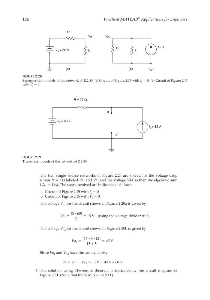
The two single source networks of Figure 2.20 are solved for the voltage drop
across R = 5 Ω labeled Va 1 and Va 2 and the voltage Vaa’ is then the algebraic sum
(Va 1 + Va 2 ). The steps involved are indicated as follows:
a. Circuit of Figure 2.15 with I s = 0
b. Circuit of Figure 2.15 with V s = 0
The voltage Va 1 for the circuit shown in Figure 2.20a is given by
Va 1
20
15
ϭ
ϭ
(5 * 60)
V (using the voltage divider rule)
The voltage Va 2 for the circuit shown in Figure 2.20b is given by
Va 2
15 5
45
ϭ
ϩ
ϭ
(15 * 5 * 12)
V
Since Va 1 and Va 2 have the same polarity
Va = Va 1 + Va 2 = 15 V + 45 V= 60 V
6. The solution using Thevenin’s theorem is indicated by the circuit diagram of
Figure 2.21. (Note that the load is R L = 5 Ω.)
FIGURE 2.20
Superposition models of the network of R.2.83. (a) Circuit of Figure 2.15 with I s = 0, (b) Circuit of Figure 2.15
with V s = 0.
V s = 60 V
15
5
12 A
5
15
Va 2
Va 1
(a)
(b)
FIGURE 2.21
Thevenin’s models of the network of R.2.83.
a
a ′
V s = 60 V
I s = 12 A
R = 15 Ω
CRC_47760_CH002.indd 124
CRC_47760_CH002.indd 124
7/23/2008 1:38:40 PM
7/23/2008 1:38:40 PM
Practical MATLAB
® Applications for Engineers
The two single source networks of Figure 2.20 are solved for the voltage drop
across R = 5 Ω labeled Va 1 and Va 2 and the voltage Vaa’ is then the algebraic sum
(Va 1 + Va 2 ). The steps involved are indicated as follows:
a. Circuit of Figure 2.15 with I s = 0
b. Circuit of Figure 2.15 with V s = 0
The voltage Va 1 for the circuit shown in Figure 2.20a is given by
Va 1
20
15
ϭ
ϭ
(5 * 60)
V (using the voltage divider rule)
The voltage Va 2 for the circuit shown in Figure 2.20b is given by
Va 2
15 5
45
ϭ
ϩ
ϭ
(15 * 5 * 12)
V
Since Va 1 and Va 2 have the same polarity
Va = Va 1 + Va 2 = 15 V + 45 V= 60 V
6. The solution using Thevenin’s theorem is indicated by the circuit diagram of
Figure 2.21. (Note that the load is R L = 5 Ω.)
FIGURE 2.20
Superposition models of the network of R.2.83. (a) Circuit of Figure 2.15 with I s = 0, (b) Circuit of Figure 2.15
with V s = 0.
V s = 60 V
15
5
12 A
5
15
Va 2
Va 1
(a)
(b)
FIGURE 2.21
Thevenin’s models of the network of R.2.83.
a
a ′
V s = 60 V
I s = 12 A
R = 15 Ω
CRC_47760_CH002.indd 124
CRC_47760_CH002.indd 124
7/23/2008 1:38:40 PM
7/23/2008 1:38:40 PM