

122
Practical MATLAB
® Applications for Engineers
Then
60 V = 20I 1 − 5(−12)
60 = 20I 1 + 60
60 60
20
−
ϭ ϭ
I 1 0
Then
Vaa’ = 5 Ω ∗ 12 A = 60 V
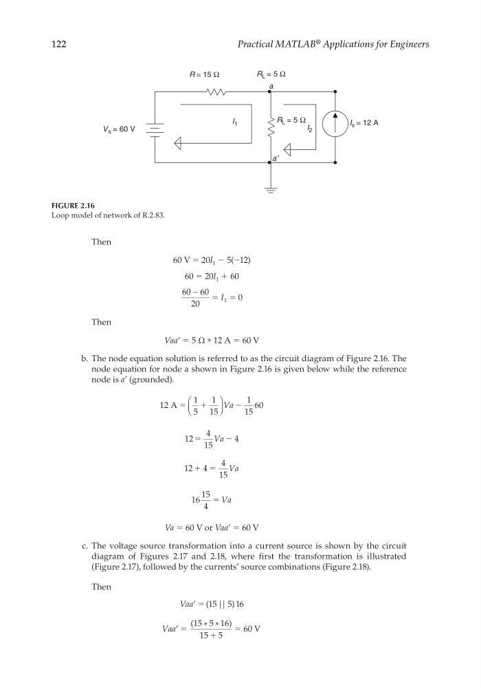
b. The node equation solution is referred to as the circuit diagram of Figure 2.16. The
node equation for node a shown in Figure 2.16 is given below while the reference
node is a’ (grounded).
12 A
60
ϭ
ϩ
1
5
1
15
1
15
Va Ϫ
12 ϭ
4
15
4
Va Ϫ
12 4
4
15
ϩ ϭ Va
16
15
4
ϭ Va
Va = 60 V or Vaa’ = 60 V
c. The voltage source transformation into a current source is shown by the circuit
diagram of Figures 2.17 and 2.18, where fi rst the transformation is illustrated
(Figure 2.17), followed by the currents’ source combinations (Figure 2.18).
Then
Vaa’ = (15 || 5) 16
Vaa′ ϭ
ϩ
ϭ
(15 * 5 * 16) 60 V
15 5
FIGURE 2.16
Loop model of network of R.2.83.
R L = 5 Ω
R L = 5 Ω
R = 15 Ω
I s = 12 A
V s = 60 V
a
a ′
I 1
I 2
CRC_47760_CH002.indd 122
CRC_47760_CH002.indd 122
7/23/2008 1:38:39 PM
7/23/2008 1:38:39 PM
Practical MATLAB
® Applications for Engineers
Then
60 V = 20I 1 − 5(−12)
60 = 20I 1 + 60
60 60
20
−
ϭ ϭ
I 1 0
Then
Vaa’ = 5 Ω ∗ 12 A = 60 V
b. The node equation solution is referred to as the circuit diagram of Figure 2.16. The
node equation for node a shown in Figure 2.16 is given below while the reference
node is a’ (grounded).
12 A
60
ϭ
ϩ
1
5
1
15
1
15
Va Ϫ
12 ϭ
4
15
4
Va Ϫ
12 4
4
15
ϩ ϭ Va
16
15
4
ϭ Va
Va = 60 V or Vaa’ = 60 V
c. The voltage source transformation into a current source is shown by the circuit
diagram of Figures 2.17 and 2.18, where fi rst the transformation is illustrated
(Figure 2.17), followed by the currents’ source combinations (Figure 2.18).
Then
Vaa’ = (15 || 5) 16
Vaa′ ϭ
ϩ
ϭ
(15 * 5 * 16) 60 V
15 5
FIGURE 2.16
Loop model of network of R.2.83.
R L = 5 Ω
R L = 5 Ω
R = 15 Ω
I s = 12 A
V s = 60 V
a
a ′
I 1
I 2
CRC_47760_CH002.indd 122
CRC_47760_CH002.indd 122
7/23/2008 1:38:39 PM
7/23/2008 1:38:39 PM