

6.2 Theory of Evaluation of Data
119
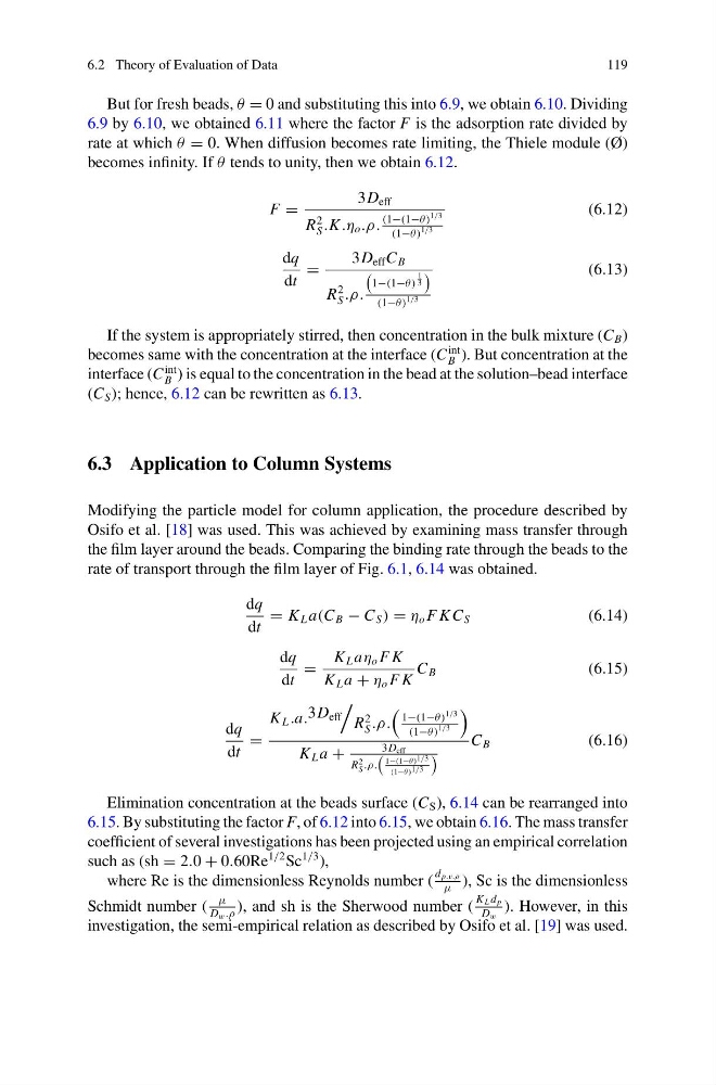
But for fresh beads, θ = 0 and substituting this into 6.9, we obtain 6.10. Dividing
6.9 by 6.10, we obtained 6.11 where the factor F is the adsorption rate divided by
rate at which θ = 0. When diffusion becomes rate limiting, the Thiele module (Ø)
becomes infinity. If θ tends to unity, then we obtain 6.12.
F =
3D eff
R
2
S .K .η o .ρ.
(1−(1−θ )
1/3
(1−θ )
1/3
(6.12)
dq
dt
=
3D eff C B
R
2
S .ρ.
1−(1−θ )
1
3
(1−θ )
1/3
(6.13)
If the system is appropriately stirred, then concentration in the bulk mixture (C B )
becomes same with the concentration at the interface (C
int
B ). But concentration at the
interface (C
int
B ) is equal to the concentration in the bead at the solution–bead interface
(C S ); hence, 6.12 can be rewritten as 6.13.
6.3 Application to Column Systems
Modifying the particle model for column application, the procedure described by
Osifo et al. [18] was used. This was achieved by examining mass transfer through
the film layer around the beads. Comparing the binding rate through the beads to the
rate of transport through the film layer of Fig. 6.1, 6.14 was obtained.
dq
dt
= K L a(C B − C S ) = η o F K C S
(6.14)
dq
dt
=
K L aη o F K
K L a + η o F K
C B
(6.15)
dq
dt
=
K L .a. 3D eff
R
2
S .ρ.
1−(1−θ )
1/3
(1−θ )
1/3
K L a +
3D eff
R
2
S .ρ.
1−(1−θ) 1/3
(1−θ) 1/3
C B
(6.16)
Elimination concentration at the beads surface (C S ), 6.14 can be rearranged into
6.15. By substituting the factor F, of 6.12 into 6.15, we obtain 6.16. The mass transfer
coefficient of several investigations has been projected using an empirical correlation
such as (sh = 2.0 + 0.60Re
1/2 Sc
1/3 ),
where Re is the dimensionless Reynolds number (
d p.v.ρ
μ
), Sc is the dimensionless
Schmidt number (
μ
D w .ρ
), and sh is the Sherwood number (
K L d p
D w
). However, in this
investigation, the semi-empirical relation as described by Osifo et al. [19] was used.
119
But for fresh beads, θ = 0 and substituting this into 6.9, we obtain 6.10. Dividing
6.9 by 6.10, we obtained 6.11 where the factor F is the adsorption rate divided by
rate at which θ = 0. When diffusion becomes rate limiting, the Thiele module (Ø)
becomes infinity. If θ tends to unity, then we obtain 6.12.
F =
3D eff
R
2
S .K .η o .ρ.
(1−(1−θ )
1/3
(1−θ )
1/3
(6.12)
dq
dt
=
3D eff C B
R
2
S .ρ.
1−(1−θ )
1
3
(1−θ )
1/3
(6.13)
If the system is appropriately stirred, then concentration in the bulk mixture (C B )
becomes same with the concentration at the interface (C
int
B ). But concentration at the
interface (C
int
B ) is equal to the concentration in the bead at the solution–bead interface
(C S ); hence, 6.12 can be rewritten as 6.13.
6.3 Application to Column Systems
Modifying the particle model for column application, the procedure described by
Osifo et al. [18] was used. This was achieved by examining mass transfer through
the film layer around the beads. Comparing the binding rate through the beads to the
rate of transport through the film layer of Fig. 6.1, 6.14 was obtained.
dq
dt
= K L a(C B − C S ) = η o F K C S
(6.14)
dq
dt
=
K L aη o F K
K L a + η o F K
C B
(6.15)
dq
dt
=
K L .a. 3D eff
R
2
S .ρ.
1−(1−θ )
1/3
(1−θ )
1/3
K L a +
3D eff
R
2
S .ρ.
1−(1−θ) 1/3
(1−θ) 1/3
C B
(6.16)
Elimination concentration at the beads surface (C S ), 6.14 can be rearranged into
6.15. By substituting the factor F, of 6.12 into 6.15, we obtain 6.16. The mass transfer
coefficient of several investigations has been projected using an empirical correlation
such as (sh = 2.0 + 0.60Re
1/2 Sc
1/3 ),
where Re is the dimensionless Reynolds number (
d p.v.ρ
μ
), Sc is the dimensionless
Schmidt number (
μ
D w .ρ
), and sh is the Sherwood number (
K L d p
D w
). However, in this
investigation, the semi-empirical relation as described by Osifo et al. [19] was used.