

173
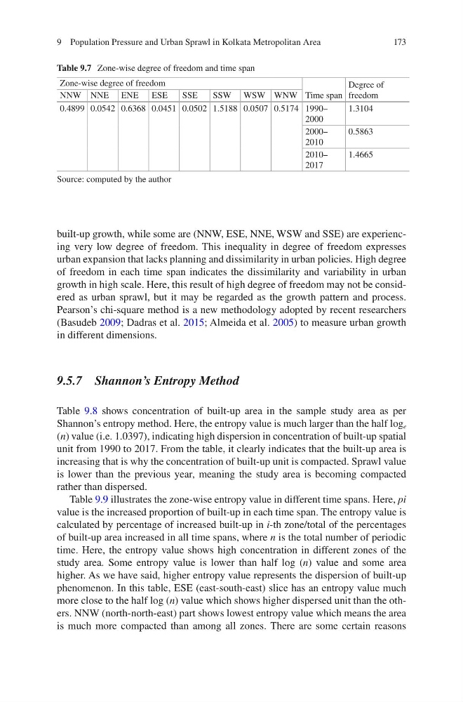
built-up growth, while some are (NNW, ESE, NNE, WSW and SSE) are experiencing very low degree of freedom. This inequality in degree of freedom expresses
urban expansion that lacks planning and dissimilarity in urban policies. High degree
of freedom in each time span indicates the dissimilarity and variability in urban
growth in high scale. Here, this result of high degree of freedom may not be considered as urban sprawl, but it may be regarded as the growth pattern and process.
Pearson’s chi-square method is a new methodology adopted by recent researchers
(Basudeb 2009; Dadras et al. 2015; Almeida et al. 2005) to measure urban growth
in different dimensions.
9.5.7 Shannon’s Entropy Method
Table 9.8 shows concentration of built-up area in the sample study area as per
Shannon’s entropy method. Here, the entropy value is much larger than the half log e
(n) value (i.e. 1.0397), indicating high dispersion in concentration of built-up spatial
unit from 1990 to 2017. From the table, it clearly indicates that the built-up area is
increasing that is why the concentration of built-up unit is compacted. Sprawl value
is lower than the previous year, meaning the study area is becoming compacted
rather than dispersed.
Table 9.9 illustrates the zone-wise entropy value in different time spans. Here, pi
value is the increased proportion of built-up in each time span. The entropy value is
calculated by percentage of increased built-up in i-th zone/total of the percentages
of built-up area increased in all time spans, where n is the total number of periodic
time. Here, the entropy value shows high concentration in different zones of the
study area. Some entropy value is lower than half log (n) value and some area
higher. As we have said, higher entropy value represents the dispersion of built-up
phenomenon. In this table, ESE (east-south-east) slice has an entropy value much
more close to the half log (n) value which shows higher dispersed unit than the others. NNW (north-north-east) part shows lowest entropy value which means the area
is much more compacted than among all zones. There are some certain reasons
Table 9.7 Zone-wise degree of freedom and time span
Zone-wise degree of freedom
Time span
Degree of
freedom
NNW NNE ENE ESE
SSE
SSW WSW WNW
0.4899 0.0542 0.6368 0.0451 0.0502 1.5188 0.0507 0.5174 1990–
2000
1.3104
2000–
2010
0.5863
2010–
2017
1.4665
Source: computed by the author
9 Population Pressure and Urban Sprawl in Kolkata Metropolitan Area
built-up growth, while some are (NNW, ESE, NNE, WSW and SSE) are experiencing very low degree of freedom. This inequality in degree of freedom expresses
urban expansion that lacks planning and dissimilarity in urban policies. High degree
of freedom in each time span indicates the dissimilarity and variability in urban
growth in high scale. Here, this result of high degree of freedom may not be considered as urban sprawl, but it may be regarded as the growth pattern and process.
Pearson’s chi-square method is a new methodology adopted by recent researchers
(Basudeb 2009; Dadras et al. 2015; Almeida et al. 2005) to measure urban growth
in different dimensions.
9.5.7 Shannon’s Entropy Method
Table 9.8 shows concentration of built-up area in the sample study area as per
Shannon’s entropy method. Here, the entropy value is much larger than the half log e
(n) value (i.e. 1.0397), indicating high dispersion in concentration of built-up spatial
unit from 1990 to 2017. From the table, it clearly indicates that the built-up area is
increasing that is why the concentration of built-up unit is compacted. Sprawl value
is lower than the previous year, meaning the study area is becoming compacted
rather than dispersed.
Table 9.9 illustrates the zone-wise entropy value in different time spans. Here, pi
value is the increased proportion of built-up in each time span. The entropy value is
calculated by percentage of increased built-up in i-th zone/total of the percentages
of built-up area increased in all time spans, where n is the total number of periodic
time. Here, the entropy value shows high concentration in different zones of the
study area. Some entropy value is lower than half log (n) value and some area
higher. As we have said, higher entropy value represents the dispersion of built-up
phenomenon. In this table, ESE (east-south-east) slice has an entropy value much
more close to the half log (n) value which shows higher dispersed unit than the others. NNW (north-north-east) part shows lowest entropy value which means the area
is much more compacted than among all zones. There are some certain reasons
Table 9.7 Zone-wise degree of freedom and time span
Zone-wise degree of freedom
Time span
Degree of
freedom
NNW NNE ENE ESE
SSE
SSW WSW WNW
0.4899 0.0542 0.6368 0.0451 0.0502 1.5188 0.0507 0.5174 1990–
2000
1.3104
2000–
2010
0.5863
2010–
2017
1.4665
Source: computed by the author
9 Population Pressure and Urban Sprawl in Kolkata Metropolitan Area