

81
Detection of Epileptic Seizure Using STFT and Statistical Analysis
DOI: http://dx.doi.org/10.5772/intechopen.89026
or negative values in non-periodical signals. In the analyses, the most basic mean
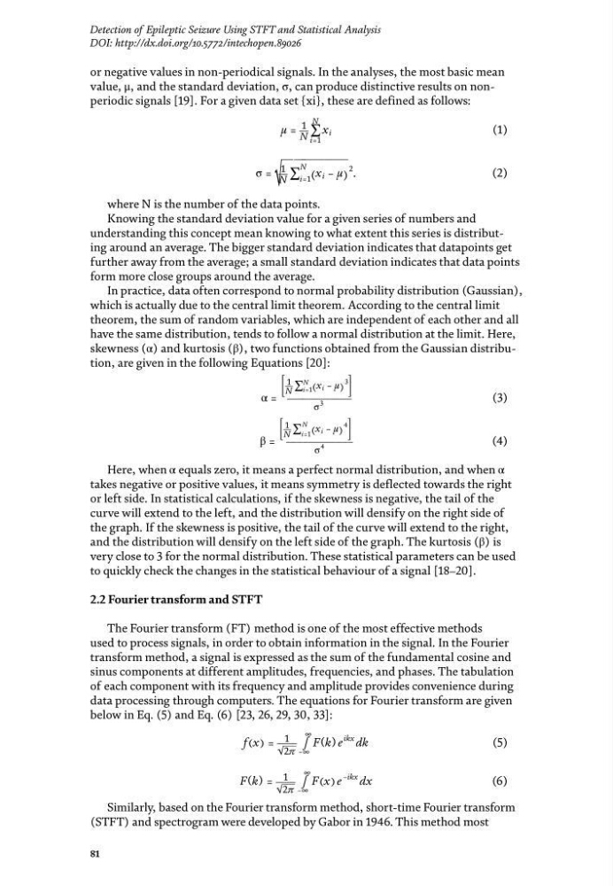
value, μ, and the standard deviation, σ, can produce distinctive results on nonperiodic signals [19]. For a given data set {xi}, these are defined as follows:
μ = 1
_
N
∑
i=1
N
x i
(1)
σ =
√
__ __ ________
1
_
N
∑ i=1
N ( x i − μ )
2
.
(2)
where N is the number of the data points.
Knowing the standard deviation value for a given series of numbers and
understanding this concept mean knowing to what extent this series is distributing around an average. The bigger standard deviation indicates that datapoints get
further away from the average; a small standard deviation indicates that data points
form more close groups around the average.
In practice, data often correspond to normal probability distribution (Gaussian),
which is actually due to the central limit theorem. According to the central limit
theorem, the sum of random variables, which are independent of each other and all
have the same distribution, tends to follow a normal distribution at the limit. Here,
skewness (α) and kurtosis (β), two functions obtained from the Gaussian distribution, are given in the following Equations [20]:
α =
[
1
_
N
∑ i=1
N ( x i − μ )
3
]
____________
σ
3
(3)
β =
[
1
_
N
∑ i=1
N ( x i − μ )
4
]
____________
σ
4
(4)
Here, when α equals zero, it means a perfect normal distribution, and when α
takes negative or positive values, it means symmetry is deflected towards the right
or left side. In statistical calculations, if the skewness is negative, the tail of the
curve will extend to the left, and the distribution will densify on the right side of
the graph. If the skewness is positive, the tail of the curve will extend to the right,
and the distribution will densify on the left side of the graph. The kurtosis (β) is
very close to 3 for the normal distribution. These statistical parameters can be used
to quickly check the changes in the statistical behaviour of a signal [18–20].
2.2 Fourier transform and STFT
The Fourier transform (FT) method is one of the most effective methods
used to process signals, in order to obtain information in the signal. In the Fourier
transform method, a signal is expressed as the sum of the fundamental cosine and
sinus components at different amplitudes, frequencies, and phases. The tabulation
of each component with its frequency and amplitude provides convenience during
data processing through computers. The equations for Fourier transform are given
below in Eq. (5) and Eq. (6) [23, 26, 29, 30, 33]:
f (x) = 1
_
√
_
2π
∫
−∞
∞
F (k) e
ikx dk
(5)
F (k) = 1
_
√
_
2π
∫
−∞
∞
F (x) e
−ikx dx
(6)
Similarly, based on the Fourier transform method, short-time Fourier transform
(STFT) and spectrogram were developed by Gabor in 1946. This method most
Detection of Epileptic Seizure Using STFT and Statistical Analysis
DOI: http://dx.doi.org/10.5772/intechopen.89026
or negative values in non-periodical signals. In the analyses, the most basic mean
value, μ, and the standard deviation, σ, can produce distinctive results on nonperiodic signals [19]. For a given data set {xi}, these are defined as follows:
μ = 1
_
N
∑
i=1
N
x i
(1)
σ =
√
__ __ ________
1
_
N
∑ i=1
N ( x i − μ )
2
.
(2)
where N is the number of the data points.
Knowing the standard deviation value for a given series of numbers and
understanding this concept mean knowing to what extent this series is distributing around an average. The bigger standard deviation indicates that datapoints get
further away from the average; a small standard deviation indicates that data points
form more close groups around the average.
In practice, data often correspond to normal probability distribution (Gaussian),
which is actually due to the central limit theorem. According to the central limit
theorem, the sum of random variables, which are independent of each other and all
have the same distribution, tends to follow a normal distribution at the limit. Here,
skewness (α) and kurtosis (β), two functions obtained from the Gaussian distribution, are given in the following Equations [20]:
α =
[
1
_
N
∑ i=1
N ( x i − μ )
3
]
____________
σ
3
(3)
β =
[
1
_
N
∑ i=1
N ( x i − μ )
4
]
____________
σ
4
(4)
Here, when α equals zero, it means a perfect normal distribution, and when α
takes negative or positive values, it means symmetry is deflected towards the right
or left side. In statistical calculations, if the skewness is negative, the tail of the
curve will extend to the left, and the distribution will densify on the right side of
the graph. If the skewness is positive, the tail of the curve will extend to the right,
and the distribution will densify on the left side of the graph. The kurtosis (β) is
very close to 3 for the normal distribution. These statistical parameters can be used
to quickly check the changes in the statistical behaviour of a signal [18–20].
2.2 Fourier transform and STFT
The Fourier transform (FT) method is one of the most effective methods
used to process signals, in order to obtain information in the signal. In the Fourier
transform method, a signal is expressed as the sum of the fundamental cosine and
sinus components at different amplitudes, frequencies, and phases. The tabulation
of each component with its frequency and amplitude provides convenience during
data processing through computers. The equations for Fourier transform are given
below in Eq. (5) and Eq. (6) [23, 26, 29, 30, 33]:
f (x) = 1
_
√
_
2π
∫
−∞
∞
F (k) e
ikx dk
(5)
F (k) = 1
_
√
_
2π
∫
−∞
∞
F (x) e
−ikx dx
(6)
Similarly, based on the Fourier transform method, short-time Fourier transform
(STFT) and spectrogram were developed by Gabor in 1946. This method most