

from physics and biological vision, as introduced by [12]. The underlying idea is to
account for the multiscale nature of real-world objects, which implies that objects
may be perceived in different ways depending on the scale of observation. Taken to
the limit, a scale-space representation furthermore considers representations at all
scales simultaneously. Scale spaces have been introduced independently in Japan
and Europe by [12, 13]. The axiomatic linear scale-space theory was formalized in
series of works by Witkin [14] and Koenderink [15].
Scale-space approaches are ubiquitous in feature detection/description, as well
as dense correspondence mapping (e.g., large-offset optical flow is typically done in
coarse-to-fine fashion) [9].
5.1 The Gaussian scale space
The liner scale-space theory provides a systematic way of dealing with spatially
uncorrelated Gaussian noise. A fundamental result of scale-space theory states that
if some general conditions are imposed on the types of computations that are to be
performed in the earliest stages of visual processing, then convolution by the
Gaussian kernel and its derivatives provides a canonical class of image operators
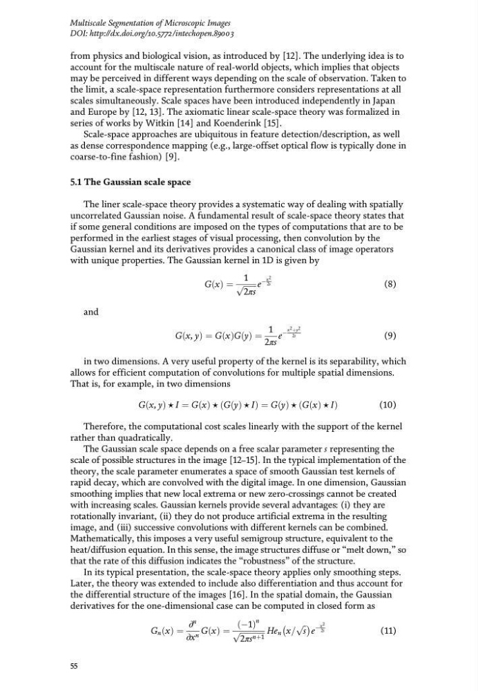
with unique properties. The Gaussian kernel in 1D is given by
Gx ð Þ¼
1
ffiffiffiffiffiffi ffi
2πs
p
e
�
x 2
2s
(8)
and
G x, y
ð Þ¼Gx ðÞ Gy ð Þ¼
1
2πs
e
�
x 2 þy 2
2s
(9)
in two dimensions. A very useful property of the kernel is its separability, which
allows for efficient computation of convolutions for multiple spatial dimensions.
That is, for example, in two dimensions
G x, y
ðÞ ⋆ I ¼ Gx ðÞ ⋆ Gy ðÞ⋆ I
ð
Þ¼Gy ðÞ⋆ Gx ðÞ ⋆ I
ðÞ
(10)
Therefore, the computational cost scales linearly with the support of the kernel
rather than quadratically.
The Gaussian scale space depends on a free scalar parameter s representing the
scale of possible structures in the image [12–15]. In the typical implementation of the
theory, the scale parameter enumerates a space of smooth Gaussian test kernels of
rapid decay, which are convolved with the digital image. In one dimension, Gaussian
smoothing implies that new local extrema or new zero-crossings cannot be created
with increasing scales. Gaussian kernels provide several advantages: (i) they are
rotationally invariant, (ii) they do not produce artificial extrema in the resulting
image, and (iii) successive convolutions with different kernels can be combined.
Mathematically, this imposes a very useful semigroup structure, equivalent to the
heat/diffusion equation. In this sense, the image structures diffuse or “melt down,” so
that the rate of this diffusion indicates the “robustness” of the structure.
In its typical presentation, the scale-space theory applies only smoothing steps.
Later, the theory was extended to include also differentiation and thus account for
the differential structure of the images [16]. In the spatial domain, the Gaussian
derivatives for the one-dimensional case can be computed in closed form as
G n x
ð Þ¼
∂
n
∂x n Gx ð Þ¼
�1
ðÞ
n
ffiffiffiffiffiffiffiffiffiffiffiffiffi
2πs nþ1
p
He n x=
ffiffi
s
p
��
e
�
x 2
2s
(11)
55
Multiscale Segmentation of Microscopic Images
DOI: http://dx.doi.org/10.5772/intechopen.89003
account for the multiscale nature of real-world objects, which implies that objects
may be perceived in different ways depending on the scale of observation. Taken to
the limit, a scale-space representation furthermore considers representations at all
scales simultaneously. Scale spaces have been introduced independently in Japan
and Europe by [12, 13]. The axiomatic linear scale-space theory was formalized in
series of works by Witkin [14] and Koenderink [15].
Scale-space approaches are ubiquitous in feature detection/description, as well
as dense correspondence mapping (e.g., large-offset optical flow is typically done in
coarse-to-fine fashion) [9].
5.1 The Gaussian scale space
The liner scale-space theory provides a systematic way of dealing with spatially
uncorrelated Gaussian noise. A fundamental result of scale-space theory states that
if some general conditions are imposed on the types of computations that are to be
performed in the earliest stages of visual processing, then convolution by the
Gaussian kernel and its derivatives provides a canonical class of image operators
with unique properties. The Gaussian kernel in 1D is given by
Gx ð Þ¼
1
ffiffiffiffiffiffi ffi
2πs
p
e
�
x 2
2s
(8)
and
G x, y
ð Þ¼Gx ðÞ Gy ð Þ¼
1
2πs
e
�
x 2 þy 2
2s
(9)
in two dimensions. A very useful property of the kernel is its separability, which
allows for efficient computation of convolutions for multiple spatial dimensions.
That is, for example, in two dimensions
G x, y
ðÞ ⋆ I ¼ Gx ðÞ ⋆ Gy ðÞ⋆ I
ð
Þ¼Gy ðÞ⋆ Gx ðÞ ⋆ I
ðÞ
(10)
Therefore, the computational cost scales linearly with the support of the kernel
rather than quadratically.
The Gaussian scale space depends on a free scalar parameter s representing the
scale of possible structures in the image [12–15]. In the typical implementation of the
theory, the scale parameter enumerates a space of smooth Gaussian test kernels of
rapid decay, which are convolved with the digital image. In one dimension, Gaussian
smoothing implies that new local extrema or new zero-crossings cannot be created
with increasing scales. Gaussian kernels provide several advantages: (i) they are
rotationally invariant, (ii) they do not produce artificial extrema in the resulting
image, and (iii) successive convolutions with different kernels can be combined.
Mathematically, this imposes a very useful semigroup structure, equivalent to the
heat/diffusion equation. In this sense, the image structures diffuse or “melt down,” so
that the rate of this diffusion indicates the “robustness” of the structure.
In its typical presentation, the scale-space theory applies only smoothing steps.
Later, the theory was extended to include also differentiation and thus account for
the differential structure of the images [16]. In the spatial domain, the Gaussian
derivatives for the one-dimensional case can be computed in closed form as
G n x
ð Þ¼
∂
n
∂x n Gx ð Þ¼
�1
ðÞ
n
ffiffiffiffiffiffiffiffiffiffiffiffiffi
2πs nþ1
p
He n x=
ffiffi
s
p
��
e
�
x 2
2s
(11)
55
Multiscale Segmentation of Microscopic Images
DOI: http://dx.doi.org/10.5772/intechopen.89003