

22
H. Schlör et al.
Table 8 Key model parameters
Country
A
B
C
D
Interest rate (%)
5
5
5
5
Time preference rate (%)
5
5
5
5
Steady-state growth rate (%)
−0.001
1.2
1.9
−1.3
Labour development (%)
0.001
0.001
0.001
0.001
Source Authors (2020) and IEK-STE/SRH (2020)
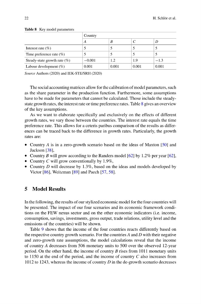
The social accounting matrices allow for the calibration of model parameters, such
as the share parameter in the production function. Furthermore, some assumptions
have to be made for parameters that cannot be calculated. Those include the steadystate growth rates, the interest rate or time preference rates. Table 8 gives an overview
of the key assumptions.
As we want to elaborate specifically and exclusively on the effects of different
growth rates, we vary those between the countries. The interest rate equals the time
preference rate. This allows for a ceteris paribus comparison of the results as differences can be traced back to the difference in growth rates. Particularly, the growth
rates are:
• Country A is in a zero-growth scenario based on the ideas of Maxton [50] and
Jackson [38],
• Country B will grow according to the Randers model [62] by 1.2% per year [62],
• Country C will grow conventionally by 1.9%,
• Country D will decrease by 1.3%, based on the ideas and models developed by
Victor [86], Weitzman [89] and Paech [57, 58].
5 Model Results
In the following, the results of our stylized economic model for the four countries will
be presented. The impact of our four scenarios and its economic framework conditions on the FEW nexus sector and on the other economic indicators (i.e. income,
consumption, savings, investments, gross output, trade relations, utility level and the
emissions of the countries) will be shown.
Table 9 shows that the income of the four countries reacts differently based on
the respective country growth scenario. For the countries A and D with their negative
and zero-growth rate assumptions, the model calculations reveal that the income
of country A decreases from 506 monetary units to 500 over the observed 12-year
period. On the other hand, the income of country B rises from 1011 monetary units
to 1150 at the end of the period, and the income of country C also increases from
1012 to 1243, whereas the income of country D in the de-growth scenario decreases
H. Schlör et al.
Table 8 Key model parameters
Country
A
B
C
D
Interest rate (%)
5
5
5
5
Time preference rate (%)
5
5
5
5
Steady-state growth rate (%)
−0.001
1.2
1.9
−1.3
Labour development (%)
0.001
0.001
0.001
0.001
Source Authors (2020) and IEK-STE/SRH (2020)
The social accounting matrices allow for the calibration of model parameters, such
as the share parameter in the production function. Furthermore, some assumptions
have to be made for parameters that cannot be calculated. Those include the steadystate growth rates, the interest rate or time preference rates. Table 8 gives an overview
of the key assumptions.
As we want to elaborate specifically and exclusively on the effects of different
growth rates, we vary those between the countries. The interest rate equals the time
preference rate. This allows for a ceteris paribus comparison of the results as differences can be traced back to the difference in growth rates. Particularly, the growth
rates are:
• Country A is in a zero-growth scenario based on the ideas of Maxton [50] and
Jackson [38],
• Country B will grow according to the Randers model [62] by 1.2% per year [62],
• Country C will grow conventionally by 1.9%,
• Country D will decrease by 1.3%, based on the ideas and models developed by
Victor [86], Weitzman [89] and Paech [57, 58].
5 Model Results
In the following, the results of our stylized economic model for the four countries will
be presented. The impact of our four scenarios and its economic framework conditions on the FEW nexus sector and on the other economic indicators (i.e. income,
consumption, savings, investments, gross output, trade relations, utility level and the
emissions of the countries) will be shown.
Table 9 shows that the income of the four countries reacts differently based on
the respective country growth scenario. For the countries A and D with their negative
and zero-growth rate assumptions, the model calculations reveal that the income
of country A decreases from 506 monetary units to 500 over the observed 12-year
period. On the other hand, the income of country B rises from 1011 monetary units
to 1150 at the end of the period, and the income of country C also increases from
1012 to 1243, whereas the income of country D in the de-growth scenario decreases