

Reflections About the Food–Energy–Water Nexus in a World …
19
The model equations that describe the optimal behaviour of all agents are
explained in the next subsection, while the database and calibration of relevant parameters will be discussed afterwards. The database does not describe the economic
situation of a real country. Instead, we chose a fictive database for two reasons:
• First, this paper is not a forecast for a particular country but aims a revealing
essential mechanisms correlated to different growth scenarios.
• Second, the stylized model approach was chosen to reveal the effects of the
different growth strategies without disturbing side effects such as the Lehman
crash 2008, the Euro crises 2012, or the current Corona caused economic
shutdowns 2020.
4.2 The Model
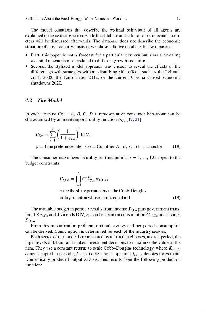
In each country Co = A, B, C, D a representative consumer behaviour can be
characterized by an intertemporal utility function U Co [17, 21]
U Co =
∞
t=1
1
1 + ϕ Co
t
ln U t ,
ϕ = time preference rate, Co = Countries A, B, C, D, i = sector
(18)
The consumer maximizes its utility for time periods t = 1, …, 12 subject to the
budget constraints
U t,Co =
3
i=1
C
α Hi
t,i,Co , α H,Co,i
α are the share parameters in the Cobb-Douglas
utility function whose sum is equal to 1
(19)
The available budget in period t results from income Y t,Co plus government transfers TRF t,Co and dividends DIV t,Co can be spent on consumption C t,i,Co and savings
S t,Co .
From this maximization problem, optimal savings and per period consumption
can be derived. Consumption is determined for each of the industry sectors.
Each sector of our model is represented by a firm that chooses, at each period, the
input levels of labour and makes investment decisions to maximize the value of the
firm. They use a constant returns to scale Cobb–Douglas technology, where K t,i,Co
denotes capital in period t, L t,i,Co is the labour input and I t,i,Co denotes investment.
Domestically produced output XD t,i,Co thus results from the following production
function:
19
The model equations that describe the optimal behaviour of all agents are
explained in the next subsection, while the database and calibration of relevant parameters will be discussed afterwards. The database does not describe the economic
situation of a real country. Instead, we chose a fictive database for two reasons:
• First, this paper is not a forecast for a particular country but aims a revealing
essential mechanisms correlated to different growth scenarios.
• Second, the stylized model approach was chosen to reveal the effects of the
different growth strategies without disturbing side effects such as the Lehman
crash 2008, the Euro crises 2012, or the current Corona caused economic
shutdowns 2020.
4.2 The Model
In each country Co = A, B, C, D a representative consumer behaviour can be
characterized by an intertemporal utility function U Co [17, 21]
U Co =
∞
t=1
1
1 + ϕ Co
t
ln U t ,
ϕ = time preference rate, Co = Countries A, B, C, D, i = sector
(18)
The consumer maximizes its utility for time periods t = 1, …, 12 subject to the
budget constraints
U t,Co =
3
i=1
C
α Hi
t,i,Co , α H,Co,i
α are the share parameters in the Cobb-Douglas
utility function whose sum is equal to 1
(19)
The available budget in period t results from income Y t,Co plus government transfers TRF t,Co and dividends DIV t,Co can be spent on consumption C t,i,Co and savings
S t,Co .
From this maximization problem, optimal savings and per period consumption
can be derived. Consumption is determined for each of the industry sectors.
Each sector of our model is represented by a firm that chooses, at each period, the
input levels of labour and makes investment decisions to maximize the value of the
firm. They use a constant returns to scale Cobb–Douglas technology, where K t,i,Co
denotes capital in period t, L t,i,Co is the labour input and I t,i,Co denotes investment.
Domestically produced output XD t,i,Co thus results from the following production
function: