

14
H. Schlör et al.
C 1 = S 0 (1 + r )
S 0 =
C 1
(1 + r )
I = I 0 = C 0 +
C 1
(1 + r )
(8)
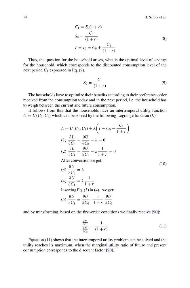
Thus, the question for the household arises, what is the optimal level of savings
for the household, which corresponds to the discounted consumption level of the
next period C 1 expressed in Eq. (9).
S 0 =
C 1
(1 + r )
(9)
The households have to optimize their benefits according to their preference order
received from the consumption today and in the next period, i.e. the household has
to weigh between the current and future consumption.
It follows from this that the households have an intertemporal utility function
U = U (C 0 , C 1 ) which can be solved by the following Lagrange function (L):
L = U (C 0 , C 1 ) + λ
I − C 0 −
C 1
1 + r
(1)
∂ L
∂C 0
=
∂U
∂C 0
− λ = 0
(2)
∂ L
∂C 1
=
∂U
∂C 1
− λ
1
1 + r
= 0
After conversion we get:
(3)
∂U
∂C 0
= λ
(4)
∂U
∂C 1
= λ
1
1 + r
Inserting Eq. (3) in (4), we get:
(5)
∂U
∂C 1
=
∂U
∂C 0
·
1
1 + r
∂U
∂C 0
(10)
and by transforming, based on the first-order conditions we finally receive [90]:
∂U
∂C 1
∂U
∂C 0
=
1
(1 + r )
(11)
Equation (11) shows that the intertemporal utility problem can be solved and the
utility reaches its maximum, when the marginal utility ratio of future and present
consumption corresponds to the discount factor [90].
H. Schlör et al.
C 1 = S 0 (1 + r )
S 0 =
C 1
(1 + r )
I = I 0 = C 0 +
C 1
(1 + r )
(8)
Thus, the question for the household arises, what is the optimal level of savings
for the household, which corresponds to the discounted consumption level of the
next period C 1 expressed in Eq. (9).
S 0 =
C 1
(1 + r )
(9)
The households have to optimize their benefits according to their preference order
received from the consumption today and in the next period, i.e. the household has
to weigh between the current and future consumption.
It follows from this that the households have an intertemporal utility function
U = U (C 0 , C 1 ) which can be solved by the following Lagrange function (L):
L = U (C 0 , C 1 ) + λ
I − C 0 −
C 1
1 + r
(1)
∂ L
∂C 0
=
∂U
∂C 0
− λ = 0
(2)
∂ L
∂C 1
=
∂U
∂C 1
− λ
1
1 + r
= 0
After conversion we get:
(3)
∂U
∂C 0
= λ
(4)
∂U
∂C 1
= λ
1
1 + r
Inserting Eq. (3) in (4), we get:
(5)
∂U
∂C 1
=
∂U
∂C 0
·
1
1 + r
∂U
∂C 0
(10)
and by transforming, based on the first-order conditions we finally receive [90]:
∂U
∂C 1
∂U
∂C 0
=
1
(1 + r )
(11)
Equation (11) shows that the intertemporal utility problem can be solved and the
utility reaches its maximum, when the marginal utility ratio of future and present
consumption corresponds to the discount factor [90].