

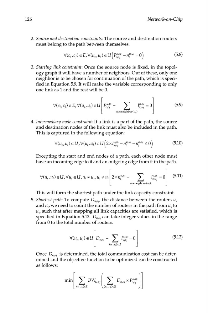
2. Source and destination constraints: The source and destination routers
must belong to the path between themselves.
∀(c i , c j )∈E,∀( u , u )∈U ( P
usut
− n
usut
s
t
s
= 0 )
(5.8)
cicj
3. Starting link constraint: Once the source node is fixed, in the topology graph it will have a number of neighbors. Out of these, only one
neighbor is to be chosen for continuation of the path, which is specified in Equation 5.9. It will make the variable corresponding to only
one link as 1 and the rest will be 0.
⎡ ⎡
⎤
∀( c i ,
c j )
∈E,∀(
u s ,
u )
∈
U
P
usut
usut
t
⎢
⎢
ci cj −
∑
l u u =
0
⎥
(5.9)
s k
⎥
⎣
uk ∈ neighbor ( us )
⎦
4. Intermediary node constraint: If a link is a part of the path, the source
and destination nodes of the link must also be included in the path.
This is captured in the following equation:
∀(u , u )∈U,∀(u , u )∈U ( 2 × l
usut
− n
usut
usut
s
t
i
j
u uj
i
− n j ≤ )
(5.10)
i
0
Excepting the start and end nodes of a path, each other node must
have an incoming edge to it and an outgoing edge from it in the path.
⎡
⎤
∀( u s , u t )∈U, ∀u i ∈U, u u
usut
u ut
( .11)
i ≠
s
5
s , u i ≠ u t ⎢ 2 × n
⎢
i
−
l
⎥
ui u
0
⎣
uj∈
∑ j = ⎥
neighbor r(ui )
⎦
This will form the shortest path under the link capacity constraint.
5. Shortest path: To compute D us ut , the distance between the routers u s
and u t , we need to count the number of routers in the path from u s to
u t , such that after mapping all link capacities are satisfied, which is
specified in Equation 5.12. D us ut can take integer values in the range
from 0 to the total number of routers.
⎡
⎤
∀( u , u )
∈
U ⎢ D −
∑
l
usut
⎥
5
s
t
( .12)
⎢
usut
ui uj =
0
⎥
⎣
(ui ,uj )∈ U
⎦
Once D us ut is determined, the total communication cost can be determined and the objective function to be optimized can be constructed
as follows:
⎡
⎛
⎞ ⎤
min ⎢
∑
BW
usut ⎥
⎢
ci ,cj ⎜
D
⎜
us ut ×
P c i c ⎟
j
⎟ ⎥
⎣
( ci , c j )∈ E
∑
⎝
(us , ut )∈ U
⎠
⎦ ⎦
126
Network-on-Chip
must belong to the path between themselves.
∀(c i , c j )∈E,∀( u , u )∈U ( P
usut
− n
usut
s
t
s
= 0 )
(5.8)
cicj
3. Starting link constraint: Once the source node is fixed, in the topology graph it will have a number of neighbors. Out of these, only one
neighbor is to be chosen for continuation of the path, which is specified in Equation 5.9. It will make the variable corresponding to only
one link as 1 and the rest will be 0.
⎡ ⎡
⎤
∀( c i ,
c j )
∈E,∀(
u s ,
u )
∈
U
P
usut
usut
t
⎢
⎢
ci cj −
∑
l u u =
0
⎥
(5.9)
s k
⎥
⎣
uk ∈ neighbor ( us )
⎦
4. Intermediary node constraint: If a link is a part of the path, the source
and destination nodes of the link must also be included in the path.
This is captured in the following equation:
∀(u , u )∈U,∀(u , u )∈U ( 2 × l
usut
− n
usut
usut
s
t
i
j
u uj
i
− n j ≤ )
(5.10)
i
0
Excepting the start and end nodes of a path, each other node must
have an incoming edge to it and an outgoing edge from it in the path.
⎡
⎤
∀( u s , u t )∈U, ∀u i ∈U, u u
usut
u ut
( .11)
i ≠
s
5
s , u i ≠ u t ⎢ 2 × n
⎢
i
−
l
⎥
ui u
0
⎣
uj∈
∑ j = ⎥
neighbor r(ui )
⎦
This will form the shortest path under the link capacity constraint.
5. Shortest path: To compute D us ut , the distance between the routers u s
and u t , we need to count the number of routers in the path from u s to
u t , such that after mapping all link capacities are satisfied, which is
specified in Equation 5.12. D us ut can take integer values in the range
from 0 to the total number of routers.
⎡
⎤
∀( u , u )
∈
U ⎢ D −
∑
l
usut
⎥
5
s
t
( .12)
⎢
usut
ui uj =
0
⎥
⎣
(ui ,uj )∈ U
⎦
Once D us ut is determined, the total communication cost can be determined and the objective function to be optimized can be constructed
as follows:
⎡
⎛
⎞ ⎤
min ⎢
∑
BW
usut ⎥
⎢
ci ,cj ⎜
D
⎜
us ut ×
P c i c ⎟
j
⎟ ⎥
⎣
( ci , c j )∈ E
∑
⎝
(us , ut )∈ U
⎠
⎦ ⎦
126
Network-on-Chip