

192
J. Prakash et al.
ρ
dV
dt
= div ϒ + f + ρ e E x ,
(3)
(c
ρ) f
dT
dt
= α m ∇
2 T + (c
ρ) p
D B ∇C · ∇T +
D T
T m
∇T · ∇T
− ∇q r , (4)
dC
dt = D B ∇
2 C +
D T
T m
∇
2 T,
(5)
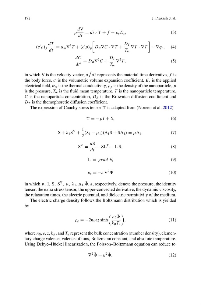
in which V is the velocity vector, d
dt represents the material time derivative, f is
the body force, c
is the volumetric volume expansion coefficient, E x is the applied
electrical field, α m is the thermal conductivity, ρ p is the density of the nanoparticle, p
is the pressure, T m is the fluid mean temperature, T is the nanoparticle temperature,
C is the nanoparticle concentration, D B is the Brownian diffusion coefficient and
D T is the themophoretic diffusion coefficient.
The expression of Cauchy stress tensor ϒ is adapted from (Noreen et al. 2012)
ϒ = −pI + S,
(6)
S + λ 1 S
∇
+
1
2
(λ 1 − μ 1 )(A 1 S + SA 1 ) = μA 1 ,
(7)
S
∇
=
dS
dt
− SL
T
− L S,
(8)
L = grad V,
(9)
ρ e = −ε ∇
2 ¯
(10)
in which p, I, S, S
∇
, μ, λ 1 , μ 1 , ¯
, ε, respectively, denote the pressure, the identity
tensor, the extra stress tensor, the upper-convected derivative, the dynamic viscosity,
the relaxation times, the electric potential, and dielectric permittivity of the medium.
The electric charge density follows the Boltzmann distribution which is yielded
by
ρ e = −2n 0 ez sinh
ez ¯
k B T n
,
(11)
where n 0 , e, z, k B , and T n represent the bulk concentration (number density), elementary charge valence, valence of ions, Boltzmann constant, and absolute temperature.
Using Debye–Hückel linearization, the Poisson–Boltzmann equation can reduce to
∇
2 ¯
= κ
2 ¯
,
(12)
J. Prakash et al.
ρ
dV
dt
= div ϒ + f + ρ e E x ,
(3)
(c
ρ) f
dT
dt
= α m ∇
2 T + (c
ρ) p
D B ∇C · ∇T +
D T
T m
∇T · ∇T
− ∇q r , (4)
dC
dt = D B ∇
2 C +
D T
T m
∇
2 T,
(5)
in which V is the velocity vector, d
dt represents the material time derivative, f is
the body force, c
is the volumetric volume expansion coefficient, E x is the applied
electrical field, α m is the thermal conductivity, ρ p is the density of the nanoparticle, p
is the pressure, T m is the fluid mean temperature, T is the nanoparticle temperature,
C is the nanoparticle concentration, D B is the Brownian diffusion coefficient and
D T is the themophoretic diffusion coefficient.
The expression of Cauchy stress tensor ϒ is adapted from (Noreen et al. 2012)
ϒ = −pI + S,
(6)
S + λ 1 S
∇
+
1
2
(λ 1 − μ 1 )(A 1 S + SA 1 ) = μA 1 ,
(7)
S
∇
=
dS
dt
− SL
T
− L S,
(8)
L = grad V,
(9)
ρ e = −ε ∇
2 ¯
(10)
in which p, I, S, S
∇
, μ, λ 1 , μ 1 , ¯
, ε, respectively, denote the pressure, the identity
tensor, the extra stress tensor, the upper-convected derivative, the dynamic viscosity,
the relaxation times, the electric potential, and dielectric permittivity of the medium.
The electric charge density follows the Boltzmann distribution which is yielded
by
ρ e = −2n 0 ez sinh
ez ¯
k B T n
,
(11)
where n 0 , e, z, k B , and T n represent the bulk concentration (number density), elementary charge valence, valence of ions, Boltzmann constant, and absolute temperature.
Using Debye–Hückel linearization, the Poisson–Boltzmann equation can reduce to
∇
2 ¯
= κ
2 ¯
,
(12)