

Agents in Economic Markets and Games
131
S u p p l y
D e m a n d
P r i c e
( i n d e p e n d e n t
v a r i a b l e )
Q u a n t i t y ( d e p e n d e n t v a r i a b l e )
E
P e
Q e
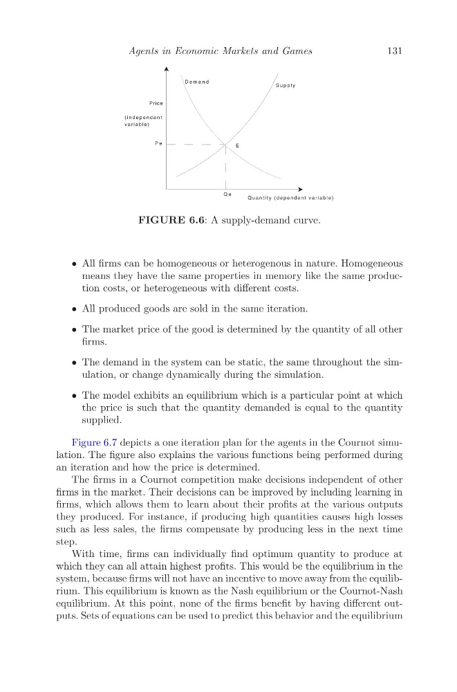
FIGURE 6.6: A supply-demand curve.
• All firms can be homogeneous or heterogenous in nature. Homogeneous
means they have the same properties in memory like the same production costs, or heterogeneous with different costs.
• All produced goods are sold in the same iteration.
• The market price of the good is determined by the quantity of all other
firms.
• The demand in the system can be static, the same throughout the simulation, or change dynamically during the simulation.
• The model exhibits an equilibrium which is a particular point at which
the price is such that the quantity demanded is equal to the quantity
supplied.
Figure 6.7 depicts a one iteration plan for the agents in the Cournot simulation. The figure also explains the various functions being performed during
an iteration and how the price is determined.
The firms in a Cournot competition make decisions independent of other
firms in the market. Their decisions can be improved by including learning in
firms, which allows them to learn about their profits at the various outputs
they produced. For instance, if producing high quantities causes high losses
such as less sales, the firms compensate by producing less in the next time
step.
With time, firms can individually find optimum quantity to produce at
which they can all attain highest profits. This would be the equilibrium in the
system, because firms will not have an incentive to move away from the equilibrium. This equilibrium is known as the Nash equilibrium or the Cournot-Nash
equilibrium. At this point, none of the firms benefit by having different outputs. Sets of equations can be used to predict this behavior and the equilibrium
131
S u p p l y
D e m a n d
P r i c e
( i n d e p e n d e n t
v a r i a b l e )
Q u a n t i t y ( d e p e n d e n t v a r i a b l e )
E
P e
Q e
FIGURE 6.6: A supply-demand curve.
• All firms can be homogeneous or heterogenous in nature. Homogeneous
means they have the same properties in memory like the same production costs, or heterogeneous with different costs.
• All produced goods are sold in the same iteration.
• The market price of the good is determined by the quantity of all other
firms.
• The demand in the system can be static, the same throughout the simulation, or change dynamically during the simulation.
• The model exhibits an equilibrium which is a particular point at which
the price is such that the quantity demanded is equal to the quantity
supplied.
Figure 6.7 depicts a one iteration plan for the agents in the Cournot simulation. The figure also explains the various functions being performed during
an iteration and how the price is determined.
The firms in a Cournot competition make decisions independent of other
firms in the market. Their decisions can be improved by including learning in
firms, which allows them to learn about their profits at the various outputs
they produced. For instance, if producing high quantities causes high losses
such as less sales, the firms compensate by producing less in the next time
step.
With time, firms can individually find optimum quantity to produce at
which they can all attain highest profits. This would be the equilibrium in the
system, because firms will not have an incentive to move away from the equilibrium. This equilibrium is known as the Nash equilibrium or the Cournot-Nash
equilibrium. At this point, none of the firms benefit by having different outputs. Sets of equations can be used to predict this behavior and the equilibrium