

M-SERVE and P-SERVE
63
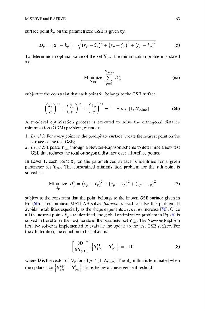
surface point ˆ
x p on the parametrized GSE is given by:
D p = =x p − ˆ
x p =
x p − ˆ
x p
2 +
y p − ˆ
y p
2 +
z p − ˆ
z p
2
(5)
To determine an optimal value of the set Y par , the minimization problem is stated
as:
Minimize
Y par
N points
p=1
D
2
p
(6a)
subject to the constraint that each point ˆ
x p belongs to the GSE surface
¯
x p
a
n 1
+
¯
y p
b
n 2
+
¯
z p
c
n 3
= 1 ∀ p ∈ [1, N points ]
(6b)
A two-level optimization process is executed to solve the orthogonal distance
minimization (ODM) problem, given as:
1. Level 1: For every point on the precipitate surface, locate the nearest point on the
surface of the test GSE;
2. Level 2: Update Y par through a Newton-Raphson scheme to determine a new test
GSE that reduces the total orthogonal distance over all surface points.
In Level 1, each point ¯
x p on the parametrized surface is identified for a given
parameter set Y par . The constrained minimization problem for the pth point is
solved as:
Minimize
ˆ
x p
D
2
p =
x p − ˆ
x p
2 +
y p − ˆ
y p
2 +
z p − ˆ
z p
2
(7)
subject to the constraint that the point belongs to the known GSE surface given in
Eq. (6b). The nonlinear MATLAB solver fmincon is used to solve this problem. It
avoids instabilities especially as the shape exponents n 1 , n 2 , n 3 increase [50]. Once
all the nearest points ˆ
x p are identified, the global optimization problem in Eq. (6) is
solved in Level 2 for the next iterate of the parameter set Y par . The Newton-Raphson
iterative solver is implemented to evaluate the update to the test GSE surface. For
the ith iteration, the equation to be solved is:
∂D
∂Y par
i
Y
i+1
par − Y
i
par
= −D
i
(8)
where D is the vector of D p for all p ∈ [1, N slice ]. The algorithm is terminated when
the update size
Y i+1
par − Y i
par
drops below a convergence threshold.
63
surface point ˆ
x p on the parametrized GSE is given by:
D p = =x p − ˆ
x p =
x p − ˆ
x p
2 +
y p − ˆ
y p
2 +
z p − ˆ
z p
2
(5)
To determine an optimal value of the set Y par , the minimization problem is stated
as:
Minimize
Y par
N points
p=1
D
2
p
(6a)
subject to the constraint that each point ˆ
x p belongs to the GSE surface
¯
x p
a
n 1
+
¯
y p
b
n 2
+
¯
z p
c
n 3
= 1 ∀ p ∈ [1, N points ]
(6b)
A two-level optimization process is executed to solve the orthogonal distance
minimization (ODM) problem, given as:
1. Level 1: For every point on the precipitate surface, locate the nearest point on the
surface of the test GSE;
2. Level 2: Update Y par through a Newton-Raphson scheme to determine a new test
GSE that reduces the total orthogonal distance over all surface points.
In Level 1, each point ¯
x p on the parametrized surface is identified for a given
parameter set Y par . The constrained minimization problem for the pth point is
solved as:
Minimize
ˆ
x p
D
2
p =
x p − ˆ
x p
2 +
y p − ˆ
y p
2 +
z p − ˆ
z p
2
(7)
subject to the constraint that the point belongs to the known GSE surface given in
Eq. (6b). The nonlinear MATLAB solver fmincon is used to solve this problem. It
avoids instabilities especially as the shape exponents n 1 , n 2 , n 3 increase [50]. Once
all the nearest points ˆ
x p are identified, the global optimization problem in Eq. (6) is
solved in Level 2 for the next iterate of the parameter set Y par . The Newton-Raphson
iterative solver is implemented to evaluate the update to the test GSE surface. For
the ith iteration, the equation to be solved is:
∂D
∂Y par
i
Y
i+1
par − Y
i
par
= −D
i
(8)
where D is the vector of D p for all p ∈ [1, N slice ]. The algorithm is terminated when
the update size
Y i+1
par − Y i
par
drops below a convergence threshold.