

354
A. Agrawal et al.
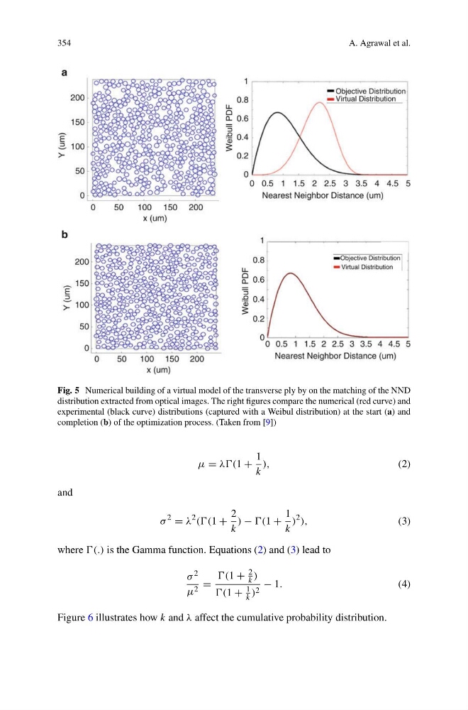
Fig. 5 Numerical building of a virtual model of the transverse ply by on the matching of the NND
distribution extracted from optical images. The right figures compare the numerical (red curve) and
experimental (black curve) distributions (captured with a Weibul distribution) at the start (a) and
completion (b) of the optimization process. (Taken from [9])
μ = λλ(1 +
1
k
),
(2)
and
σ
2
= λ
2 (((1 +
2
k
) − (1 +
1
k
)
2 ),
(3)
where (.) is the Gamma function. Equations (2) and (3) lead to
σ 2
μ 2 =
(1 +
2
k )
(1 +
1
k ) 2
− 1.
(4)
Figure 6 illustrates how k and λ affect the cumulative probability distribution.
A. Agrawal et al.
Fig. 5 Numerical building of a virtual model of the transverse ply by on the matching of the NND
distribution extracted from optical images. The right figures compare the numerical (red curve) and
experimental (black curve) distributions (captured with a Weibul distribution) at the start (a) and
completion (b) of the optimization process. (Taken from [9])
μ = λλ(1 +
1
k
),
(2)
and
σ
2
= λ
2 (((1 +
2
k
) − (1 +
1
k
)
2 ),
(3)
where (.) is the Gamma function. Equations (2) and (3) lead to
σ 2
μ 2 =
(1 +
2
k )
(1 +
1
k ) 2
− 1.
(4)
Figure 6 illustrates how k and λ affect the cumulative probability distribution.