

184
J. Hochhalter et al.
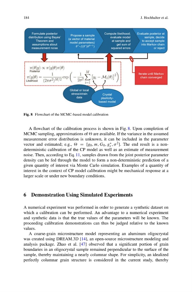
Fig. 8 Flowchart of the MCMC-based model calibration
A flowchart of the calibration process is shown in Fig. 8. Upon completion of
MCMC sampling, approximations of are available. If the variance in the assumed
measurement error distribution is unknown, it can be included in the parameter
vector and estimated; e.g., = [g 0 , m, G 0 , g ∗
s , σ 2 ]. The end result is a nondeterministic calibration of the CP model as well as an estimate of measurement
noise. Then, according to Eq. 11, samples drawn from the joint posterior parameter
density can be fed through the model to form a non-deterministic prediction of a
given quantity of interest via Monte Carlo simulation. Examples of a quantity of
interest in the context of CP model calibration might be mechanical response at a
larger scale or under new boundary conditions.
6 Demonstration Using Simulated Experiments
A numerical experiment was performed in order to generate a synthetic dataset on
which a calibration can be performed. An advantage to a numerical experiment
and synthetic data is that the true values of the parameters will be known. The
proceeding calibration demonstrations can thus be judged relative to the known
values.
A coarse-grain microstructure model representing an aluminum oligocrystal
was created using DREAM.3D [14], an open-source microstructure modeling and
analysis package. Zhao et al. [47] observed that a significant portion of grain
boundaries in an oligocrystal sample remained perpendicular to the surface of the
sample, thereby maintaining a nearly columnar shape. For simplicity, an idealized
perfectly columnar grain structure is considered in the current study, thereby
J. Hochhalter et al.
Fig. 8 Flowchart of the MCMC-based model calibration
A flowchart of the calibration process is shown in Fig. 8. Upon completion of
MCMC sampling, approximations of are available. If the variance in the assumed
measurement error distribution is unknown, it can be included in the parameter
vector and estimated; e.g., = [g 0 , m, G 0 , g ∗
s , σ 2 ]. The end result is a nondeterministic calibration of the CP model as well as an estimate of measurement
noise. Then, according to Eq. 11, samples drawn from the joint posterior parameter
density can be fed through the model to form a non-deterministic prediction of a
given quantity of interest via Monte Carlo simulation. Examples of a quantity of
interest in the context of CP model calibration might be mechanical response at a
larger scale or under new boundary conditions.
6 Demonstration Using Simulated Experiments
A numerical experiment was performed in order to generate a synthetic dataset on
which a calibration can be performed. An advantage to a numerical experiment
and synthetic data is that the true values of the parameters will be known. The
proceeding calibration demonstrations can thus be judged relative to the known
values.
A coarse-grain microstructure model representing an aluminum oligocrystal
was created using DREAM.3D [14], an open-source microstructure modeling and
analysis package. Zhao et al. [47] observed that a significant portion of grain
boundaries in an oligocrystal sample remained perpendicular to the surface of the
sample, thereby maintaining a nearly columnar shape. For simplicity, an idealized
perfectly columnar grain structure is considered in the current study, thereby