

182
J. Hochhalter et al.
for i = 1, . . . , M, where Y i , , and ε i are random variables representing
the measurements, model parameters, and measurement errors, respectively. In
the context of the CP model calibration herein, = [g 0 , m, G 0 , g ∗
s ] and the
measurements are local or global observations, as discussed in previous sections.
M is the total number of measurements available, and M i (() denotes the model
response corresponding to a time and location, represented by i, at which the
measurements were obtained.
The goal of model calibration is to solve the inverse problem posed by Eq. 11;
that is, determine the probability distribution of the model parameters given a set
of measurements. Formally, this involves determining the posterior density, π(θ|y),
where y and θ are realizations of the random variables Y and , respectively. Using
Bayes’ theorem, the posterior density can be expressed as:
π(θ|y) =
π(y|θ)π(θ)
π(y)
=
π(y|θ)π(θ)
R p π(y|θ)π(θ)dθ
.
(12)
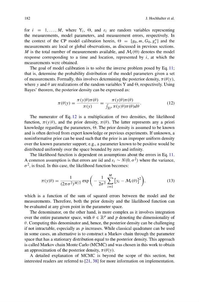
The numerator of Eq. 12 is a multiplication of two densities, the likelihood
function, π(y|θ), and the prior density, π(θ). The latter represents any a priori
knowledge regarding the parameters, . The prior density is assumed to be known
and is often derived from expert knowledge or previous experiments. If unknown, a
noninformative prior can be used such that the prior is an improper uniform density
over the known parameter support; e.g., a parameter known to be positive would be
distributed uniformly over the space bounded by zero and infinity.
The likelihood function is dependent on assumptions about the errors in Eq. 11.
A common assumption is that errors are iid and ε i ∼ N(0, σ 2 ) where the variance,
σ 2 , is fixed. In this case, the likelihood function becomes:
π(y|θ) =
1
(2πσ 2 ) M/2 exp
−
1
2σ 2
M
i=1
y i − M i (θ )
2
,
(13)
which is a function of the sum of squared errors between the model and the
measurements. Therefore, both the prior density and the likelihood function can
be evaluated at any given point in the parameter space.
The denominator, on the other hand, is more complex as it involves integration
over the entire parameter space, with θ ∈ R p and p denoting the dimensionality of
θ. Computing this denominator and, hence, the posterior density can be challenging
if not intractable, especially as p increases. While classical quadrature can be used
in some cases, an alternative is to construct a Markov chain through the parameter
space that has a stationary distribution equal to the posterior density. This approach
is called Markov chain Monte Carlo (MCMC) and was chosen in this work to obtain
an approximation of the posterior density, π(θ|y).
A detailed explanation of MCMC is beyond the scope of this section, but
interested readers are referred to [21, 38] for more information on implementation.
J. Hochhalter et al.
for i = 1, . . . , M, where Y i , , and ε i are random variables representing
the measurements, model parameters, and measurement errors, respectively. In
the context of the CP model calibration herein, = [g 0 , m, G 0 , g ∗
s ] and the
measurements are local or global observations, as discussed in previous sections.
M is the total number of measurements available, and M i (() denotes the model
response corresponding to a time and location, represented by i, at which the
measurements were obtained.
The goal of model calibration is to solve the inverse problem posed by Eq. 11;
that is, determine the probability distribution of the model parameters given a set
of measurements. Formally, this involves determining the posterior density, π(θ|y),
where y and θ are realizations of the random variables Y and , respectively. Using
Bayes’ theorem, the posterior density can be expressed as:
π(θ|y) =
π(y|θ)π(θ)
π(y)
=
π(y|θ)π(θ)
R p π(y|θ)π(θ)dθ
.
(12)
The numerator of Eq. 12 is a multiplication of two densities, the likelihood
function, π(y|θ), and the prior density, π(θ). The latter represents any a priori
knowledge regarding the parameters, . The prior density is assumed to be known
and is often derived from expert knowledge or previous experiments. If unknown, a
noninformative prior can be used such that the prior is an improper uniform density
over the known parameter support; e.g., a parameter known to be positive would be
distributed uniformly over the space bounded by zero and infinity.
The likelihood function is dependent on assumptions about the errors in Eq. 11.
A common assumption is that errors are iid and ε i ∼ N(0, σ 2 ) where the variance,
σ 2 , is fixed. In this case, the likelihood function becomes:
π(y|θ) =
1
(2πσ 2 ) M/2 exp
−
1
2σ 2
M
i=1
y i − M i (θ )
2
,
(13)
which is a function of the sum of squared errors between the model and the
measurements. Therefore, both the prior density and the likelihood function can
be evaluated at any given point in the parameter space.
The denominator, on the other hand, is more complex as it involves integration
over the entire parameter space, with θ ∈ R p and p denoting the dimensionality of
θ. Computing this denominator and, hence, the posterior density can be challenging
if not intractable, especially as p increases. While classical quadrature can be used
in some cases, an alternative is to construct a Markov chain through the parameter
space that has a stationary distribution equal to the posterior density. This approach
is called Markov chain Monte Carlo (MCMC) and was chosen in this work to obtain
an approximation of the posterior density, π(θ|y).
A detailed explanation of MCMC is beyond the scope of this section, but
interested readers are referred to [21, 38] for more information on implementation.