

176
J. Hochhalter et al.
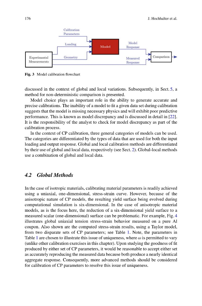
Fig. 3 Model calibration flowchart
discussed in the context of global and local variations. Subsequently, in Sect. 5, a
method for non-deterministic comparison is presented.
Model choice plays an important role in the ability to generate accurate and
precise calibrations. The inability of a model to fit a given data set during calibration
suggests that the model is missing necessary physics and will exhibit poor predictive
performance. This is known as model discrepancy and is discussed in detail in [22].
It is the responsibility of the analyst to check for model discrepancy as part of the
calibration process.
In the context of CP calibration, three general categories of models can be used.
The categories are differentiated by the types of data that are used for both the input
loading and output response. Global and local calibration methods are differentiated
by their use of global and local data, respectively (see Sect. 2). Global-local methods
use a combination of global and local data.
4.2 Global Methods
In the case of isotropic materials, calibrating material parameters is readily achieved
using a uniaxial, one-dimensional, stress-strain curve. However, because of the
anisotropic nature of CP models, the resulting yield surface being evolved during
computational simulation is six-dimensional. In the case of anisotropic material
models, as is the focus here, the reduction of a six-dimensional yield surface to a
measured scalar (one-dimensional) surface can be problematic. For example, Fig. 4
illustrates global uniaxial tension stress-strain behavior measured on a pure Al
coupon. Also shown are the computed stress-strain results, using a Taylor model,
from two disparate sets of CP parameters; see Table 1. Note, the parameters in
Table 1 are chosen to illustrate this issue of uniqueness, where ω is permitted to vary
(unlike other calibration exercises in this chapter). Upon studying the goodness of fit
produced by either set of CP parameters, it would be reasonable to accept either set
as accurately reproducing the measured data because both produce a nearly identical
aggregate response. Consequently, more advanced methods should be considered
for calibration of CP parameters to resolve this issue of uniqueness.
J. Hochhalter et al.
Fig. 3 Model calibration flowchart
discussed in the context of global and local variations. Subsequently, in Sect. 5, a
method for non-deterministic comparison is presented.
Model choice plays an important role in the ability to generate accurate and
precise calibrations. The inability of a model to fit a given data set during calibration
suggests that the model is missing necessary physics and will exhibit poor predictive
performance. This is known as model discrepancy and is discussed in detail in [22].
It is the responsibility of the analyst to check for model discrepancy as part of the
calibration process.
In the context of CP calibration, three general categories of models can be used.
The categories are differentiated by the types of data that are used for both the input
loading and output response. Global and local calibration methods are differentiated
by their use of global and local data, respectively (see Sect. 2). Global-local methods
use a combination of global and local data.
4.2 Global Methods
In the case of isotropic materials, calibrating material parameters is readily achieved
using a uniaxial, one-dimensional, stress-strain curve. However, because of the
anisotropic nature of CP models, the resulting yield surface being evolved during
computational simulation is six-dimensional. In the case of anisotropic material
models, as is the focus here, the reduction of a six-dimensional yield surface to a
measured scalar (one-dimensional) surface can be problematic. For example, Fig. 4
illustrates global uniaxial tension stress-strain behavior measured on a pure Al
coupon. Also shown are the computed stress-strain results, using a Taylor model,
from two disparate sets of CP parameters; see Table 1. Note, the parameters in
Table 1 are chosen to illustrate this issue of uniqueness, where ω is permitted to vary
(unlike other calibration exercises in this chapter). Upon studying the goodness of fit
produced by either set of CP parameters, it would be reasonable to accept either set
as accurately reproducing the measured data because both produce a nearly identical
aggregate response. Consequently, more advanced methods should be considered
for calibration of CP parameters to resolve this issue of uniqueness.