

7.2. Applications of temporal networks
91
(g) t = 7
(h) t = 8
(i) t = 9
(j) t = 10
(k) t = 11
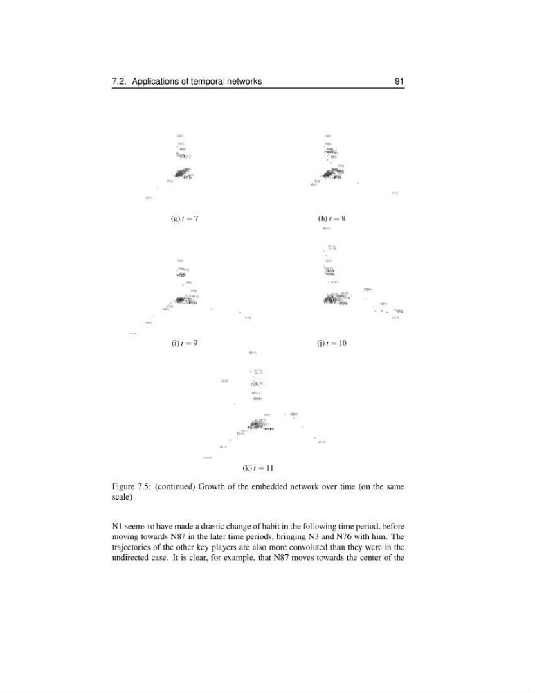
Figure 7.5: (continued) Growth of the embedded network over time (on the same
scale)
N1 seems to have made a drastic change of habit in the following time period, before
moving towards N87 in the later time periods, bringing N3 and N76 with him. The
trajectories of the other key players are also more convoluted than they were in the
undirected case. It is clear, for example, that N87 moves towards the center of the
91
(g) t = 7
(h) t = 8
(i) t = 9
(j) t = 10
(k) t = 11
Figure 7.5: (continued) Growth of the embedded network over time (on the same
scale)
N1 seems to have made a drastic change of habit in the following time period, before
moving towards N87 in the later time periods, bringing N3 and N76 with him. The
trajectories of the other key players are also more convoluted than they were in the
undirected case. It is clear, for example, that N87 moves towards the center of the