

48
Compact Models for Integrated Circuit Design
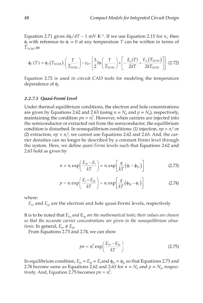
Equation 2.71 gives df f /dT ~ 1 mV K –1 . If we use Equation 2.15 for n i , then
f f with reference to f i = 0 at any temperature T can be written in terms of
T NOM as
φ
φ
f
f
NOM
NOM
kT
NOM
g
g
T
T
T
T
v
T
T
E T
kT
E
( ) = (
)
−
+ −
+
.
l n
( )
3
2
2
T T
kT
NOM
NOM
(
)
2
(2.72)
Equation 2.72 is used in circuit CAD tools for modeling the temperature
dependence of f f .
2.2.7.3 Quasi-Fermi Level
Under thermal equilibrium conditions, the electron and hole concentrations
are given by Equations 2.62 and 2.63 (using n = N d and p = N a ), respectively,
maintaining the condition pn n i
=
2 . However, when carriers are injected into
the semiconductor or extracted out from the semiconductor, the equilibrium
condition is disturbed. In nonequilibrium conditions: (1) injection, np > n i
2 or
(2) extraction, np < n i
2 , we cannot use Equations 2.62 and 2.63. And, the carrier densities can no longer be described by a constant Fermi level through
the system. Here, we define quasi-Fermi levels such that Equations 2.62 and
2.63 hold as given by
n n
E E
kT
n
q
kT
i
fn
i
i
i
fn
=
−
=
−
(
)
exp
e xp
φ φ
(2.73)
p n
E E
kT
n
q
kT
i
i
f p
i
f p
i
=
−
=
−
(
)
exp
e xp
φ
φ
(2.74)
where:
E fn and E fp are the electron and hole quasi-Fermi levels, respectively
It is to be noted that E fn and E fp are the mathematical tools; their values are chosen
so that the accurate carrier concentrations are given in the nonequilibrium situations. In general, E fn ≠ E fp .
From Equations 2.73 and 2.74, we can show
pn n
E E
kT
i
fn
fp
=
−
2 exp
(2.75)
In equilibrium condition, E fn = E fp = E f and f fn = f fp so that Equations 2.73 and
2.74 become same as Equations 2.62 and 2.63 for n = N d and p = N a , respectively. And, Equation 2.75 becomes pn n i
=
2 .
Compact Models for Integrated Circuit Design
Equation 2.71 gives df f /dT ~ 1 mV K –1 . If we use Equation 2.15 for n i , then
f f with reference to f i = 0 at any temperature T can be written in terms of
T NOM as
φ
φ
f
f
NOM
NOM
kT
NOM
g
g
T
T
T
T
v
T
T
E T
kT
E
( ) = (
)
−
+ −
+
.
l n
( )
3
2
2
T T
kT
NOM
NOM
(
)
2
(2.72)
Equation 2.72 is used in circuit CAD tools for modeling the temperature
dependence of f f .
2.2.7.3 Quasi-Fermi Level
Under thermal equilibrium conditions, the electron and hole concentrations
are given by Equations 2.62 and 2.63 (using n = N d and p = N a ), respectively,
maintaining the condition pn n i
=
2 . However, when carriers are injected into
the semiconductor or extracted out from the semiconductor, the equilibrium
condition is disturbed. In nonequilibrium conditions: (1) injection, np > n i
2 or
(2) extraction, np < n i
2 , we cannot use Equations 2.62 and 2.63. And, the carrier densities can no longer be described by a constant Fermi level through
the system. Here, we define quasi-Fermi levels such that Equations 2.62 and
2.63 hold as given by
n n
E E
kT
n
q
kT
i
fn
i
i
i
fn
=
−
=
−
(
)
exp
e xp
φ φ
(2.73)
p n
E E
kT
n
q
kT
i
i
f p
i
f p
i
=
−
=
−
(
)
exp
e xp
φ
φ
(2.74)
where:
E fn and E fp are the electron and hole quasi-Fermi levels, respectively
It is to be noted that E fn and E fp are the mathematical tools; their values are chosen
so that the accurate carrier concentrations are given in the nonequilibrium situations. In general, E fn ≠ E fp .
From Equations 2.73 and 2.74, we can show
pn n
E E
kT
i
fn
fp
=
−
2 exp
(2.75)
In equilibrium condition, E fn = E fp = E f and f fn = f fp so that Equations 2.73 and
2.74 become same as Equations 2.62 and 2.63 for n = N d and p = N a , respectively. And, Equation 2.75 becomes pn n i
=
2 .