

414
Compact Models for Integrated Circuit Design
With reference to Figure 11.27, the base current in SGP BJT model can be
obtained from Equation 11.52 as
I
I
V
v
C I
V
n v
B
SS
FM
BE
kT
SS
BE
E kT
=
−
+
−
β
exp
e xp
1
1
2
+
−
+
I
V
v
C I
V
n v
SS
RM
BC
kT
SS
BC
C kT
β
exp
exp
1
4
−
1
(11.116)
and the collector current is given by
I
I
q
V
v
V
v
I
V
C
SS
b
BE
kT
BC
kT
SS
RM
BC
=
−
+
exp
e xp
exp
β
v v
C I
V
n v
kT
SS
BC
C kT
−
−
−
1
1
4
exp
(11.117)
The corresponding model equations as implemented in SPICE are as follows:
I
IS
V
n v
ISE
V
n v
B
eff
F
BE
F kT
eff
BE
E kT
=
−
+
β
exp
e xp
1
−
+
−
+
1
1
IS
V
n v
ISC
V
n
eff
R
BC
R kT
eff
BC
C
β
exp
e xp
v v kT
−
1
(11.118)
and,
I
IS
q
V
n v
V
n v
IS
C
eff
b
BE
F kT
BC
R kT
eff
=
−
−
exp
e xp
β R R
BC
R kT
eff
BC
C kT
V
n v
ISC
V
n v
exp
exp
−
−
−
1
1
(11.119)
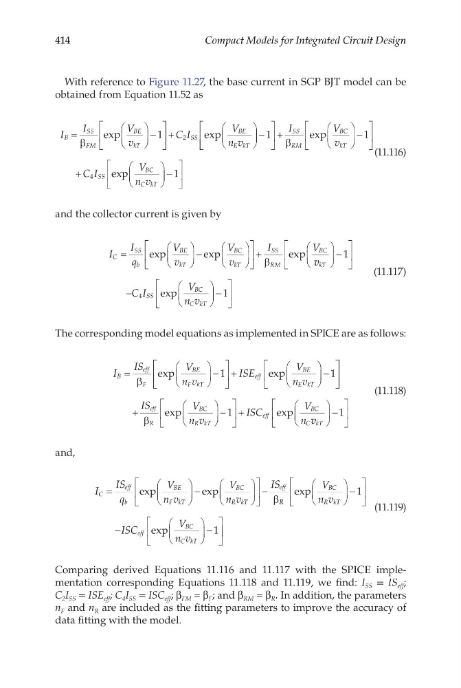
Comparing derived Equations 11.116 and 11.117 with the SPICE implementation corresponding Equations 11.118 and 11.119, we find: I SS = IS eff ;
C 2 I SS = ISE eff ; C 4 I SS = ISC eff ; β FM = β F ; and β RM = β R . In addition, the parameters
n F and n R are included as the fitting parameters to improve the accuracy of
data fitting with the model.
Compact Models for Integrated Circuit Design
With reference to Figure 11.27, the base current in SGP BJT model can be
obtained from Equation 11.52 as
I
I
V
v
C I
V
n v
B
SS
FM
BE
kT
SS
BE
E kT
=
−
+
−
β
exp
e xp
1
1
2
+
−
+
I
V
v
C I
V
n v
SS
RM
BC
kT
SS
BC
C kT
β
exp
exp
1
4
−
1
(11.116)
and the collector current is given by
I
I
q
V
v
V
v
I
V
C
SS
b
BE
kT
BC
kT
SS
RM
BC
=
−
+
exp
e xp
exp
β
v v
C I
V
n v
kT
SS
BC
C kT
−
−
−
1
1
4
exp
(11.117)
The corresponding model equations as implemented in SPICE are as follows:
I
IS
V
n v
ISE
V
n v
B
eff
F
BE
F kT
eff
BE
E kT
=
−
+
β
exp
e xp
1
−
+
−
+
1
1
IS
V
n v
ISC
V
n
eff
R
BC
R kT
eff
BC
C
β
exp
e xp
v v kT
−
1
(11.118)
and,
I
IS
q
V
n v
V
n v
IS
C
eff
b
BE
F kT
BC
R kT
eff
=
−
−
exp
e xp
β R R
BC
R kT
eff
BC
C kT
V
n v
ISC
V
n v
exp
exp
−
−
−
1
1
(11.119)
Comparing derived Equations 11.116 and 11.117 with the SPICE implementation corresponding Equations 11.118 and 11.119, we find: I SS = IS eff ;
C 2 I SS = ISE eff ; C 4 I SS = ISC eff ; β FM = β F ; and β RM = β R . In addition, the parameters
n F and n R are included as the fitting parameters to improve the accuracy of
data fitting with the model.