

22
Compact Models for Integrated Circuit Design
electron under a thermal equilibrium condition is given by the Fermi–Dirac
probability density function f(E), also called the Fermi function [1–11].
f E
E E kT
f
( )
exp
= +
−
(
)
1
1
(2.3)
where:
E f is the Fermi energy or Fermi level
k = 1.38 × 10 –23 J K –1 is the Boltzmann constant
T is the ambient temperature
The Fermi level is the energy at which the probability of finding an electron,
at any T > 0° K, is exactly one-half (Equation 2.3). From Equation 2.3, we find
that when E = E f , f(E) = 1/2, which means that the electron is equally likely to
have an energy above E f as below it. At absolute zero temperature (T = 0° K):
f(E) = 1 for E < E f , indicating that the probability of finding an electron below
E f is unity and above E f is zero (that is, f(E) = 0 for E > E f ). In other words, all
energy levels below E f are filled and all energy levels above E f are empty. At
finite temperatures, some states above E f are filled and some states below E f
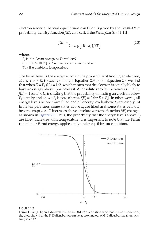
become empty. As T increases above absolute zero, the function f(E) changes
as shown in Figure 2.2. Thus, the probability that the energy levels above E f
are filled increases with temperature. It is important to note that the Fermi
function or Fermi energy applies only under equilibrium conditions.
−0.3
0.0
0.5
f(E)
1.0
F–D function
M–B function
0.0
E − E f
3 kT
0.3
FIGURE 2.2
Fermi–Dirac (F–D) and Maxwell–Boltzmann (M–B) distribution functions in a semiconductor;
the plots show that the F–D distribution can be approximated to M–B distribution at temperature, T > 3 kT.
Compact Models for Integrated Circuit Design
electron under a thermal equilibrium condition is given by the Fermi–Dirac
probability density function f(E), also called the Fermi function [1–11].
f E
E E kT
f
( )
exp
= +
−
(
)
1
1
(2.3)
where:
E f is the Fermi energy or Fermi level
k = 1.38 × 10 –23 J K –1 is the Boltzmann constant
T is the ambient temperature
The Fermi level is the energy at which the probability of finding an electron,
at any T > 0° K, is exactly one-half (Equation 2.3). From Equation 2.3, we find
that when E = E f , f(E) = 1/2, which means that the electron is equally likely to
have an energy above E f as below it. At absolute zero temperature (T = 0° K):
f(E) = 1 for E < E f , indicating that the probability of finding an electron below
E f is unity and above E f is zero (that is, f(E) = 0 for E > E f ). In other words, all
energy levels below E f are filled and all energy levels above E f are empty. At
finite temperatures, some states above E f are filled and some states below E f
become empty. As T increases above absolute zero, the function f(E) changes
as shown in Figure 2.2. Thus, the probability that the energy levels above E f
are filled increases with temperature. It is important to note that the Fermi
function or Fermi energy applies only under equilibrium conditions.
−0.3
0.0
0.5
f(E)
1.0
F–D function
M–B function
0.0
E − E f
3 kT
0.3
FIGURE 2.2
Fermi–Dirac (F–D) and Maxwell–Boltzmann (M–B) distribution functions in a semiconductor;
the plots show that the F–D distribution can be approximated to M–B distribution at temperature, T > 3 kT.