

321
Compact Models for Ultrathin Body FETs
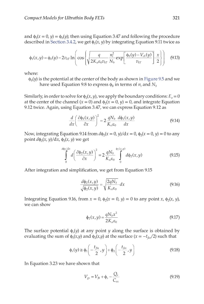
and f 1 (x = 0, y) = f 0 (y); then using Equation 3.47 and following the procedure
described in Section 3.4.2, we get f 1 (x, y) by integrating Equation 9.11 twice as
φ
φ
ε
φ
1
0
0
2
0
2
2
( , )
( )
ln cos
exp
( )
( )
x y
y
v
q
K v
n
N
y V y
v
kT
si
kT
i
b
ch
kT
=
−
−
⋅
x
2
(9.13)
where:
f 0 (y) is the potential at the center of the body as shown in Figure 9.5 and we
have used Equation 9.8 to express f B in terms of n i and N b
Similarly, in order to solve for f 2 (x, y), we apply the boundary conditions: E x = 0
at the center of the channel (x = 0) and f 2 (x = 0, y) = 0, and integrate Equation
9.12 twice. Again, using Equation 3.47, we can express Equation 9.12 as
d
dx
x y
x
qN
K
d x y
dx
b
si
∂
∂
=
φ
ε
φ
2
2
0
2
2
( , )
(, )
(9.14)
Now, integrating Equation 9.14 from df 2 (x = 0, y)/dx = 0, f 2 (x = 0, y) = 0 to any
point df 2 (x, y)/dx, f 2 (x, y) we get
d
x y
x
qN
K
d x y
d dx
b
si
x y
∂
∂
=
∫
∫
φ
ε
φ
φ
φ
2
2
0
0
2
0
2
2
2
( , )
( , )
( , )
(9.15)
After integration and simplification, we get from Equation 9.15
d x y
x y
qN
K
dx
b
si
φ
φ
ε
2
2
0
2
( , )
( , )
=
⋅
(9.16)
Integrating Equation 9.16, from x = 0, f 2 (x = 0, y) = 0 to any point x, f 2 (x, y),
we can show
φ
ε
2
2
0
2
( , )
x y
qN x
K
b
si
=
(9.17)
The surface potential f s (y) at any point y along the surface is obtained by
evaluating the sum of f 1 (x,y) and f 2 (x,y) at the surface (x = −t fin /2) such that
φ
φ
φ
s
fin
fin
y
t y
t y
( )
,
,
≅
−
+
−
1
2
2
2
(9.18)
In Equation 3.23 we have shown that
V
V
Q
C
gs
fb
s
s
ox
=
+ −
φ
(9.19)
Compact Models for Ultrathin Body FETs
and f 1 (x = 0, y) = f 0 (y); then using Equation 3.47 and following the procedure
described in Section 3.4.2, we get f 1 (x, y) by integrating Equation 9.11 twice as
φ
φ
ε
φ
1
0
0
2
0
2
2
( , )
( )
ln cos
exp
( )
( )
x y
y
v
q
K v
n
N
y V y
v
kT
si
kT
i
b
ch
kT
=
−
−
⋅
x
2
(9.13)
where:
f 0 (y) is the potential at the center of the body as shown in Figure 9.5 and we
have used Equation 9.8 to express f B in terms of n i and N b
Similarly, in order to solve for f 2 (x, y), we apply the boundary conditions: E x = 0
at the center of the channel (x = 0) and f 2 (x = 0, y) = 0, and integrate Equation
9.12 twice. Again, using Equation 3.47, we can express Equation 9.12 as
d
dx
x y
x
qN
K
d x y
dx
b
si
∂
∂
=
φ
ε
φ
2
2
0
2
2
( , )
(, )
(9.14)
Now, integrating Equation 9.14 from df 2 (x = 0, y)/dx = 0, f 2 (x = 0, y) = 0 to any
point df 2 (x, y)/dx, f 2 (x, y) we get
d
x y
x
qN
K
d x y
d dx
b
si
x y
∂
∂
=
∫
∫
φ
ε
φ
φ
φ
2
2
0
0
2
0
2
2
2
( , )
( , )
( , )
(9.15)
After integration and simplification, we get from Equation 9.15
d x y
x y
qN
K
dx
b
si
φ
φ
ε
2
2
0
2
( , )
( , )
=
⋅
(9.16)
Integrating Equation 9.16, from x = 0, f 2 (x = 0, y) = 0 to any point x, f 2 (x, y),
we can show
φ
ε
2
2
0
2
( , )
x y
qN x
K
b
si
=
(9.17)
The surface potential f s (y) at any point y along the surface is obtained by
evaluating the sum of f 1 (x,y) and f 2 (x,y) at the surface (x = −t fin /2) such that
φ
φ
φ
s
fin
fin
y
t y
t y
( )
,
,
≅
−
+
−
1
2
2
2
(9.18)
In Equation 3.23 we have shown that
V
V
Q
C
gs
fb
s
s
ox
=
+ −
φ
(9.19)