

161
Large Geometry MOSFET Compact Models
Q y
C V V
Vy
V V y
i
o x
g s
f b
B
B
s b
( )
( )
( )
= −
−
−
−
−
+
+
2
2
φ
γ φ
(4.88)
Substituting Equation 4.88 in Equation 4.64 and integrating from V(y) = V sb at
y = 0 to V(y) = V sb + V ds at y = L, we get
I
C
W
L
V V
V V
V
V
ds
s ox
g s
t h
ds
ds
ds
B
s b
=
−
−
−
+
+
(
)
µ
γ
φ
2
2
3
2
3 2
/ − −
+
(
)
2
3 2
φ B
s b
V
/
(4.89)
Equation 4.89 accounts for the bulk-charge variation in the depletion region
of MOSFETs. The linear region drain current (Equation 4.89) is sometimes
referred to as the Ihantola–Moll model [29] and used as SPICE Level 2 MOS
model. Comparing Equations 4.72 and 4.89, we find that Equation 4.89 predicts lower current compared to Equation 4.72. This is because the increasing
bulk charge Q b will reduce the inversion charge Q i for the same bias condition, resulting in a lower drain current. However, Equation 4.89 is more complex compared to Equation 4.72 and time-consuming for circuit CAD.
In order to derive model equation for I dsat , we calculate V dsat by differentiating Equation 4.89 with respect to V ds and equate the resulting expression to
zero. This results in the following expression for V dsat
V
V V
V V V
dsat
gs
fb
B
g s
f b
s b
=
−
−
+ −
−
+
+
2
2
4
2
2
φ
γ γ
γ
(4.90)
Then substituting V ds = V dsat from Equation 4.90 into Equation 4.89, we can
compute the saturation region drain current I dsat .
4.4.4.3 Square Root Approximation of Bulk-Charge Model
In order to develop a computationally efficient drain current model considering Q b (y), we simplify Equation 4.67 by Taylor series expansion and neglect
the higher order terms to get
L
V gs
Gate
V ds
X dm (y)
V sb < 0
V s = 0
Oxide
n+
n+
x dd
x sd
p-Body
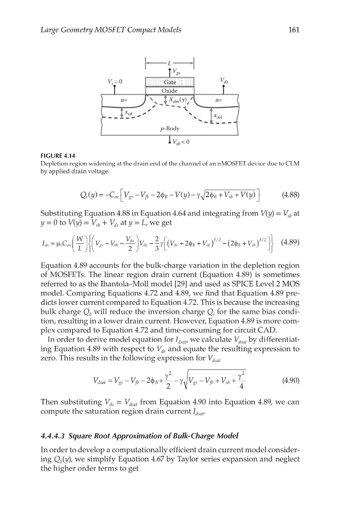
FIGURE 4.14
Depletion region widening at the drain end of the channel of an nMOSFET device due to CLM
by applied drain voltage.
Large Geometry MOSFET Compact Models
Q y
C V V
Vy
V V y
i
o x
g s
f b
B
B
s b
( )
( )
( )
= −
−
−
−
−
+
+
2
2
φ
γ φ
(4.88)
Substituting Equation 4.88 in Equation 4.64 and integrating from V(y) = V sb at
y = 0 to V(y) = V sb + V ds at y = L, we get
I
C
W
L
V V
V V
V
V
ds
s ox
g s
t h
ds
ds
ds
B
s b
=
−
−
−
+
+
(
)
µ
γ
φ
2
2
3
2
3 2
/ − −
+
(
)
2
3 2
φ B
s b
V
/
(4.89)
Equation 4.89 accounts for the bulk-charge variation in the depletion region
of MOSFETs. The linear region drain current (Equation 4.89) is sometimes
referred to as the Ihantola–Moll model [29] and used as SPICE Level 2 MOS
model. Comparing Equations 4.72 and 4.89, we find that Equation 4.89 predicts lower current compared to Equation 4.72. This is because the increasing
bulk charge Q b will reduce the inversion charge Q i for the same bias condition, resulting in a lower drain current. However, Equation 4.89 is more complex compared to Equation 4.72 and time-consuming for circuit CAD.
In order to derive model equation for I dsat , we calculate V dsat by differentiating Equation 4.89 with respect to V ds and equate the resulting expression to
zero. This results in the following expression for V dsat
V
V V
V V V
dsat
gs
fb
B
g s
f b
s b
=
−
−
+ −
−
+
+
2
2
4
2
2
φ
γ γ
γ
(4.90)
Then substituting V ds = V dsat from Equation 4.90 into Equation 4.89, we can
compute the saturation region drain current I dsat .
4.4.4.3 Square Root Approximation of Bulk-Charge Model
In order to develop a computationally efficient drain current model considering Q b (y), we simplify Equation 4.67 by Taylor series expansion and neglect
the higher order terms to get
L
V gs
Gate
V ds
X dm (y)
V sb < 0
V s = 0
Oxide
n+
n+
x dd
x sd
p-Body
FIGURE 4.14
Depletion region widening at the drain end of the channel of an nMOSFET device due to CLM
by applied drain voltage.