

205
Logic Programming and Artificial Neural Networks
y
x
0. ¯ 3
0. ¯ 3
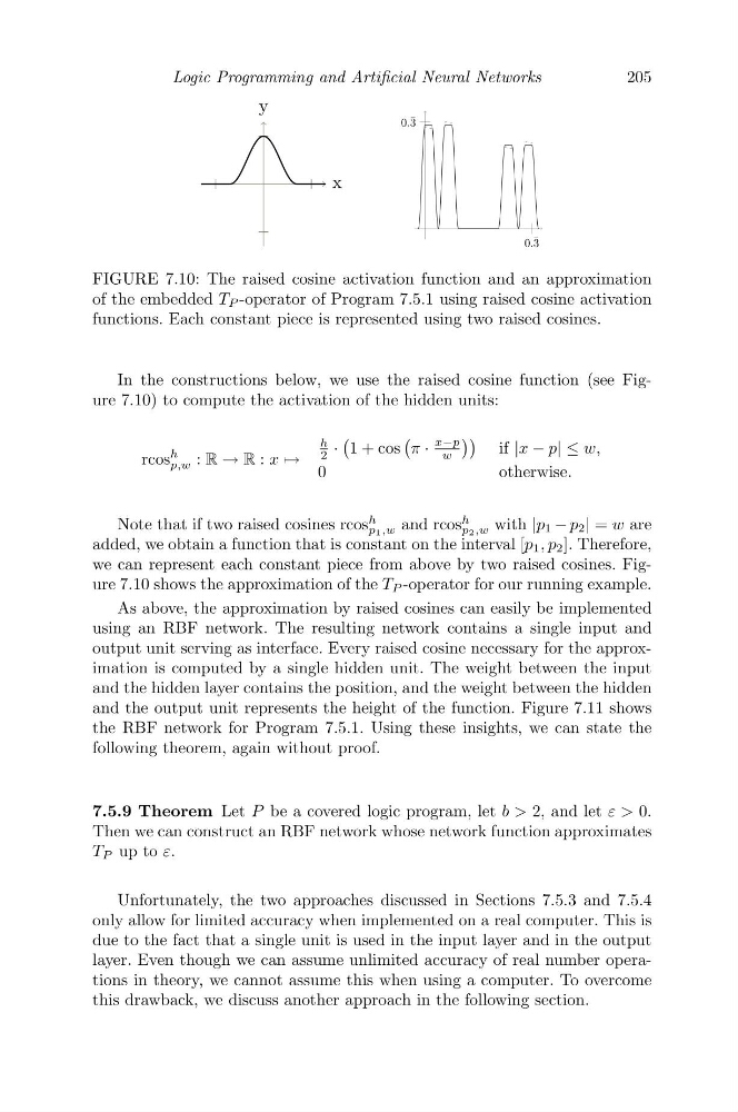
FIGURE 7.10: The raised cosine activation function and an approximation
of the embedded T P -operator of Program 7.5.1 using raised cosine activation
functions. Each constant piece is represented using two raised cosines.
In the constructions below, we use the raised cosine function (see Figure 7.10) to compute the activation of the hidden units:
A
A
bb
h
x−p
· 1 + cos π ·
if |x − p| ≤ w,
h
2
w
rcos
: R → R : x � →
p,w
0
otherwise.
Note that if two raised cosines rcos
h
and rcos
h
with |p 1 − p 2 | = w are
p1,w
p2,w
added, we obtain a function that is constant on the interval [p 1 , p 2 ]. Therefore,
we can represent each constant piece from above by two raised cosines. Figure 7.10 shows the approximation of the T P -operator for our running example.
As above, the approximation by raised cosines can easily be implemented
using an RBF network. The resulting network contains a single input and
output unit serving as interface. Every raised cosine necessary for the approximation is computed by a single hidden unit. The weight between the input
and the hidden layer contains the position, and the weight between the hidden
and the output unit represents the height of the function. Figure 7.11 shows
the RBF network for Program 7.5.1. Using these insights, we can state the
following theorem, again without proof.
7.5.9 Theorem Let P be a covered logic program, let b > 2, and let ε > 0.
Then we can construct an RBF network whose network function approximates
T P up to ε.
Unfortunately, the two approaches discussed in Sections 7.5.3 and 7.5.4
only allow for limited accuracy when implemented on a real computer. This is
due to the fact that a single unit is used in the input layer and in the output
layer. Even though we can assume unlimited accuracy of real number operations in theory, we cannot assume this when using a computer. To overcome
this drawback, we discuss another approach in the following section.
Logic Programming and Artificial Neural Networks
y
x
0. ¯ 3
0. ¯ 3
FIGURE 7.10: The raised cosine activation function and an approximation
of the embedded T P -operator of Program 7.5.1 using raised cosine activation
functions. Each constant piece is represented using two raised cosines.
In the constructions below, we use the raised cosine function (see Figure 7.10) to compute the activation of the hidden units:
A
A
bb
h
x−p
· 1 + cos π ·
if |x − p| ≤ w,
h
2
w
rcos
: R → R : x � →
p,w
0
otherwise.
Note that if two raised cosines rcos
h
and rcos
h
with |p 1 − p 2 | = w are
p1,w
p2,w
added, we obtain a function that is constant on the interval [p 1 , p 2 ]. Therefore,
we can represent each constant piece from above by two raised cosines. Figure 7.10 shows the approximation of the T P -operator for our running example.
As above, the approximation by raised cosines can easily be implemented
using an RBF network. The resulting network contains a single input and
output unit serving as interface. Every raised cosine necessary for the approximation is computed by a single hidden unit. The weight between the input
and the hidden layer contains the position, and the weight between the hidden
and the output unit represents the height of the function. Figure 7.11 shows
the RBF network for Program 7.5.1. Using these insights, we can state the
following theorem, again without proof.
7.5.9 Theorem Let P be a covered logic program, let b > 2, and let ε > 0.
Then we can construct an RBF network whose network function approximates
T P up to ε.
Unfortunately, the two approaches discussed in Sections 7.5.3 and 7.5.4
only allow for limited accuracy when implemented on a real computer. This is
due to the fact that a single unit is used in the input layer and in the output
layer. Even though we can assume unlimited accuracy of real number operations in theory, we cannot assume this when using a computer. To overcome
this drawback, we discuss another approach in the following section.