

204
Mathematical Aspects of Logic Programming Semantics
1 3 5 .9 9 4
53.864
1 3 5 .9 9 4
0 .0 1 6
-0.078
0 .0 1 6
0.5
i
−5.67
−8.98
−39.66
0.32
o
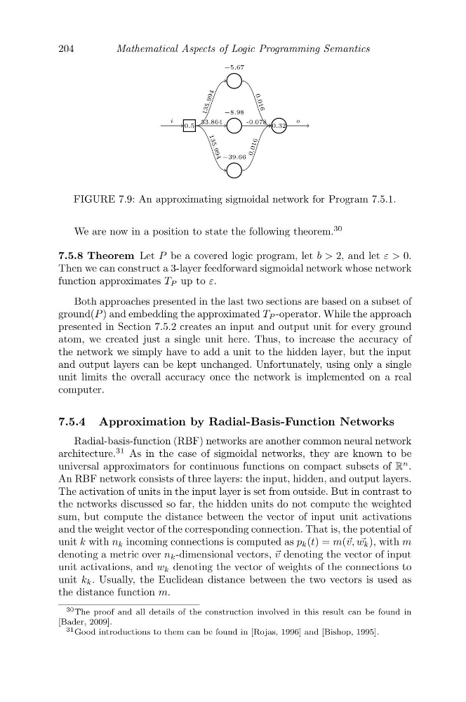
FIGURE 7.9: An approximating sigmoidal network for Program 7.5.1.
We are now in a position to state the following theorem.
30
7.5.8 Theorem Let P be a covered logic program, let b > 2, and let ε > 0.
Then we can construct a 3-layer feedforward sigmoidal network whose network
function approximates T P up to ε.
Both approaches presented in the last two sections are based on a subset of
ground(P ) and embedding the approximated T P -operator. While the approach
presented in Section 7.5.2 creates an input and output unit for every ground
atom, we created just a single unit here. Thus, to increase the accuracy of
the network we simply have to add a unit to the hidden layer, but the input
and output layers can be kept unchanged. Unfortunately, using only a single
unit limits the overall accuracy once the network is implemented on a real
computer.
7.5.4 Approximation by Radial-Basis-Function Networks
Radial-basis-function (RBF) networks are another common neural network
architecture.
31 As in the case of sigmoidal networks, they are known to be
universal approximators for continuous functions on compact subsets of R
n .
An RBF network consists of three layers: the input, hidden, and output layers.
The activation of units in the input layer is set from outside. But in contrast to
the networks discussed so far, the hidden units do not compute the weighted
sum, but compute the distance between the vector of input unit activations
and the weight vector of the corresponding connection. That is, the potential of
unit k with n k incoming connections is computed as p k (t) = m(� v, �
w k ), with m
denoting a metric over n k -dimensional vectors, � v denoting the vector of input
unit activations, and w k denoting the vector of weights of the connections to
unit k k . Usually, the Euclidean distance between the two vectors is used as
the distance function m.
30 The proof and all details of the construction involved in this result can be found in
[Bader, 2009].
31 Good introductions to them can be found in [Rojas, 1996] and [Bishop, 1995].
Mathematical Aspects of Logic Programming Semantics
1 3 5 .9 9 4
53.864
1 3 5 .9 9 4
0 .0 1 6
-0.078
0 .0 1 6
0.5
i
−5.67
−8.98
−39.66
0.32
o
FIGURE 7.9: An approximating sigmoidal network for Program 7.5.1.
We are now in a position to state the following theorem.
30
7.5.8 Theorem Let P be a covered logic program, let b > 2, and let ε > 0.
Then we can construct a 3-layer feedforward sigmoidal network whose network
function approximates T P up to ε.
Both approaches presented in the last two sections are based on a subset of
ground(P ) and embedding the approximated T P -operator. While the approach
presented in Section 7.5.2 creates an input and output unit for every ground
atom, we created just a single unit here. Thus, to increase the accuracy of
the network we simply have to add a unit to the hidden layer, but the input
and output layers can be kept unchanged. Unfortunately, using only a single
unit limits the overall accuracy once the network is implemented on a real
computer.
7.5.4 Approximation by Radial-Basis-Function Networks
Radial-basis-function (RBF) networks are another common neural network
architecture.
31 As in the case of sigmoidal networks, they are known to be
universal approximators for continuous functions on compact subsets of R
n .
An RBF network consists of three layers: the input, hidden, and output layers.
The activation of units in the input layer is set from outside. But in contrast to
the networks discussed so far, the hidden units do not compute the weighted
sum, but compute the distance between the vector of input unit activations
and the weight vector of the corresponding connection. That is, the potential of
unit k with n k incoming connections is computed as p k (t) = m(� v, �
w k ), with m
denoting a metric over n k -dimensional vectors, � v denoting the vector of input
unit activations, and w k denoting the vector of weights of the connections to
unit k k . Usually, the Euclidean distance between the two vectors is used as
the distance function m.
30 The proof and all details of the construction involved in this result can be found in
[Bader, 2009].
31 Good introductions to them can be found in [Rojas, 1996] and [Bishop, 1995].