

188
Mathematical Aspects of Logic Programming Semantics
p k (t)
w
k 1
v 1 (t)
.
.
.
w kj
v j (t)
.
.
.
w k n k
vn k (t)
v k (t + ∆t)
θ k
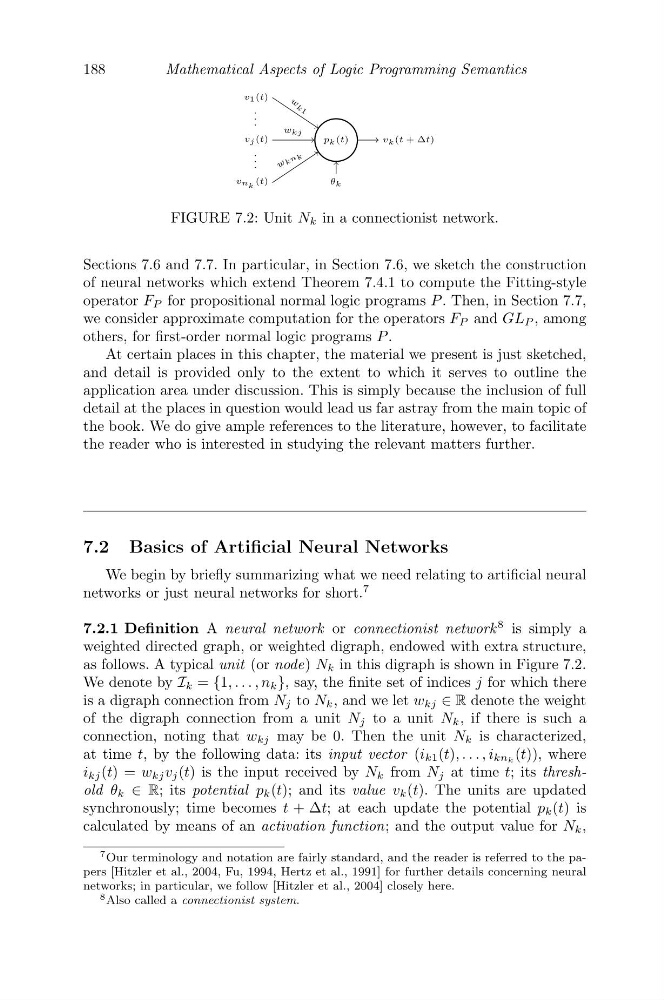
FIGURE 7.2: Unit N k in a connectionist network.
Sections 7.6 and 7.7. In particular, in Section 7.6, we sketch the construction
of neural networks which extend Theorem 7.4.1 to compute the Fitting-style
operator F P for propositional normal logic programs P . Then, in Section 7.7,
we consider approximate computation for the operators F P and GL P , among
others, for first-order normal logic programs P .
At certain places in this chapter, the material we present is just sketched,
and detail is provided only to the extent to which it serves to outline the
application area under discussion. This is simply because the inclusion of full
detail at the places in question would lead us far astray from the main topic of
the book. We do give ample references to the literature, however, to facilitate
the reader who is interested in studying the relevant matters further.
7.2 Basics of Artificial Neural Networks
We begin by briefly summarizing what we need relating to artificial neural
networks or just neural networks for short.
7
7.2.1 Definition A neural network or connectionist network
8 is simply a
weighted directed graph, or weighted digraph, endowed with extra structure,
as follows. A typical unit (or node) N k in this digraph is shown in Figure 7.2.
We denote by I k = {1, . . . , n k }, say, the finite set of indices j for which there
is a digraph connection from N j to N k , and we let w kj ∈ R denote the weight
of the digraph connection from a unit N j to a unit N k , if there is such a
connection, noting that w kj may be 0. Then the unit N k is characterized,
at time t, by the following data: its input vector (i k1 (t), . . . , i kn k (t)), where
i kj (t) = w kj v j (t) is the input received by N k from N j at time t; its threshold θ k ∈ R; its potential p k (t); and its value v k (t). The units are updated
synchronously; time becomes t + Δt; at each update the potential p k (t) is
calculated by means of an activation function; and the output value for N k ,
7 Our terminology and notation are fairly standard, and the reader is referred to the papers [Hitzler et al., 2004, Fu, 1994, Hertz et al., 1991] for further details concerning neural
networks; in particular, we follow [Hitzler et al., 2004] closely here.
8 Also called a connectionist system.
Mathematical Aspects of Logic Programming Semantics
p k (t)
w
k 1
v 1 (t)
.
.
.
w kj
v j (t)
.
.
.
w k n k
vn k (t)
v k (t + ∆t)
θ k
FIGURE 7.2: Unit N k in a connectionist network.
Sections 7.6 and 7.7. In particular, in Section 7.6, we sketch the construction
of neural networks which extend Theorem 7.4.1 to compute the Fitting-style
operator F P for propositional normal logic programs P . Then, in Section 7.7,
we consider approximate computation for the operators F P and GL P , among
others, for first-order normal logic programs P .
At certain places in this chapter, the material we present is just sketched,
and detail is provided only to the extent to which it serves to outline the
application area under discussion. This is simply because the inclusion of full
detail at the places in question would lead us far astray from the main topic of
the book. We do give ample references to the literature, however, to facilitate
the reader who is interested in studying the relevant matters further.
7.2 Basics of Artificial Neural Networks
We begin by briefly summarizing what we need relating to artificial neural
networks or just neural networks for short.
7
7.2.1 Definition A neural network or connectionist network
8 is simply a
weighted directed graph, or weighted digraph, endowed with extra structure,
as follows. A typical unit (or node) N k in this digraph is shown in Figure 7.2.
We denote by I k = {1, . . . , n k }, say, the finite set of indices j for which there
is a digraph connection from N j to N k , and we let w kj ∈ R denote the weight
of the digraph connection from a unit N j to a unit N k , if there is such a
connection, noting that w kj may be 0. Then the unit N k is characterized,
at time t, by the following data: its input vector (i k1 (t), . . . , i kn k (t)), where
i kj (t) = w kj v j (t) is the input received by N k from N j at time t; its threshold θ k ∈ R; its potential p k (t); and its value v k (t). The units are updated
synchronously; time becomes t + Δt; at each update the potential p k (t) is
calculated by means of an activation function; and the output value for N k ,
7 Our terminology and notation are fairly standard, and the reader is referred to the papers [Hitzler et al., 2004, Fu, 1994, Hertz et al., 1991] for further details concerning neural
networks; in particular, we follow [Hitzler et al., 2004] closely here.
8 Also called a connectionist system.