

Stratified halfspace
Laterally heterogeneous sphere
Laterally homogeneous sphere
v = f(r, θ, φ)
θ φ
v = f(r)
Layered halfspace
v i = f i (z)
v = f(z)
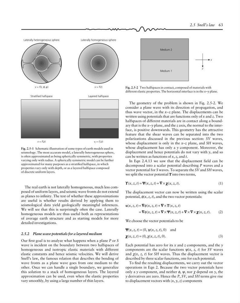
Fig. 2.5-1 Schematic illustration of some types of earth models used in
seismology. The most accurate model, a laterally heterogeneous sphere,
is often approximated as being spherically symmetric, with properties
varying only with radius. A spherically symmetric model can be further
approximated for many purposes as a stratified halfspace, in which
properties vary only with depth, or as a layered halfspace composed
of discrete uniform layers.
The real earth is not laterally homogeneous, much less composed of uniform layers, and seismic wave fronts do not extend
as planes to infinity. The test of whether these approximations
are useful is whether results derived by applying them to
seismological data yield geologically meaningful inferences.
We will see that this is surprisingly often the case. Laterally
homogeneous models are thus useful both as representations
of average earth structure and as starting models for more
detailed investigations.
2.5.2 Plane wave potentials for a layered medium
Our first goal is to analyze what happens when a plane P or S
wave is incident on the boundary between two halfspaces of
homogeneous and isotropic elastic materials with different
elastic constants and hence seismic velocities. We will derive
Snell’s law, the famous relation that describes the bending of
wave fronts as a plane wave goes from one medium to the
other. Once we can handle a single boundary, we generalize
this solution to a stack of homogeneous layers. The layered
approximation can be used, even when the elastic properties
vary smoothly, by using a large number of thin layers.
Fig. 2.5-2 Two halfspaces in contact, composed of materials with
different elastic properties. The horizontal interface is in the x–y plane.
2.5 Snell’s law 63
x
Medium 2
z
Medium 1
The geometry of the problem is shown in Fig. 2.5-2. We
consider a plane wave with its direction of propagation, and
thus wave vector, in the x–z plane. The displacements can be
written using potentials that are functions only of x and z. Two
halfspaces of different materials are in contact along a boundary that is the x–y plane, and the z axis, the normal to the interface, is positive downwards. This geometry has the attractive
feature that the shear waves can be separated into the two
polarizations discussed in the previous section: SV waves,
whose displacement is only in the x–z plane, and SH waves,
whose displacement has only a y component. Moreover, the
displacement and hence potentials do not vary with y, and so
can be written as functions of x, z, and t.
In Eqn 2.4.13 we saw that the displacement field can be
decomposed into a scalar potential describing P waves and a
vector potential for S waves. To separate the SV and SH waves,
we split the vector potential ϒ
ϒ ϒ
ϒ ϒ into two terms,
ϒ
ϒ ϒ
ϒ ϒ(x, z, t) = Ψ
Ψ Ψ
Ψ Ψ(x, z, t) + ∇
∇ ∇
∇ ∇ × χ
χ χ
χ χ(x, z, t).
(1)
The displacement vector can now be written using the scalar
potential, φ(x, z, t), and the two vector potentials:
u(x, z, t) = ∇
∇ ∇
∇ ∇φ(x, z, t) + ∇
∇ ∇
∇ ∇ × ϒ
ϒ ϒ
ϒ ϒ(x, z, t)
= ∇
∇ ∇
∇ ∇φ(x, z, t) + ∇
∇ ∇
∇ ∇ × Ψ
Ψ Ψ
Ψ Ψ(x, z, t) + ∇
∇ ∇
∇ ∇ × ∇
∇ ∇
∇ ∇ × χ
χ χ
χ χ(x, z, t).
(2)
We choose the vector potentials to be
Ψ
Ψ Ψ
Ψ Ψ(x, z, t) = (0, ψ(x, z, t), 0) and
χ
χ χ
χ χ(x, z, t) = (0, χ(x, z, t), 0).
(3)
Each potential has zero for its x and z components, and the y
components are the scalar functions ψ(x, z, t) for SV waves
and χ(x, z, t) for SH waves. Thus the displacement vector is
described by three scalar functions, one for each potential.
To find the resulting displacements, we carry out the vector
operations in Eqn 2. Because the two vector potentials have
only a y component, and neither φ, ψ, nor χ depend on y, the
y derivatives are zero. Hence the P, SV, and SH terms give rise
to displacement vectors with (x, y, z) components
Laterally heterogeneous sphere
Laterally homogeneous sphere
v = f(r, θ, φ)
θ φ
v = f(r)
Layered halfspace
v i = f i (z)
v = f(z)
Fig. 2.5-1 Schematic illustration of some types of earth models used in
seismology. The most accurate model, a laterally heterogeneous sphere,
is often approximated as being spherically symmetric, with properties
varying only with radius. A spherically symmetric model can be further
approximated for many purposes as a stratified halfspace, in which
properties vary only with depth, or as a layered halfspace composed
of discrete uniform layers.
The real earth is not laterally homogeneous, much less composed of uniform layers, and seismic wave fronts do not extend
as planes to infinity. The test of whether these approximations
are useful is whether results derived by applying them to
seismological data yield geologically meaningful inferences.
We will see that this is surprisingly often the case. Laterally
homogeneous models are thus useful both as representations
of average earth structure and as starting models for more
detailed investigations.
2.5.2 Plane wave potentials for a layered medium
Our first goal is to analyze what happens when a plane P or S
wave is incident on the boundary between two halfspaces of
homogeneous and isotropic elastic materials with different
elastic constants and hence seismic velocities. We will derive
Snell’s law, the famous relation that describes the bending of
wave fronts as a plane wave goes from one medium to the
other. Once we can handle a single boundary, we generalize
this solution to a stack of homogeneous layers. The layered
approximation can be used, even when the elastic properties
vary smoothly, by using a large number of thin layers.
Fig. 2.5-2 Two halfspaces in contact, composed of materials with
different elastic properties. The horizontal interface is in the x–y plane.
2.5 Snell’s law 63
x
Medium 2
z
Medium 1
The geometry of the problem is shown in Fig. 2.5-2. We
consider a plane wave with its direction of propagation, and
thus wave vector, in the x–z plane. The displacements can be
written using potentials that are functions only of x and z. Two
halfspaces of different materials are in contact along a boundary that is the x–y plane, and the z axis, the normal to the interface, is positive downwards. This geometry has the attractive
feature that the shear waves can be separated into the two
polarizations discussed in the previous section: SV waves,
whose displacement is only in the x–z plane, and SH waves,
whose displacement has only a y component. Moreover, the
displacement and hence potentials do not vary with y, and so
can be written as functions of x, z, and t.
In Eqn 2.4.13 we saw that the displacement field can be
decomposed into a scalar potential describing P waves and a
vector potential for S waves. To separate the SV and SH waves,
we split the vector potential ϒ
ϒ ϒ
ϒ ϒ into two terms,
ϒ
ϒ ϒ
ϒ ϒ(x, z, t) = Ψ
Ψ Ψ
Ψ Ψ(x, z, t) + ∇
∇ ∇
∇ ∇ × χ
χ χ
χ χ(x, z, t).
(1)
The displacement vector can now be written using the scalar
potential, φ(x, z, t), and the two vector potentials:
u(x, z, t) = ∇
∇ ∇
∇ ∇φ(x, z, t) + ∇
∇ ∇
∇ ∇ × ϒ
ϒ ϒ
ϒ ϒ(x, z, t)
= ∇
∇ ∇
∇ ∇φ(x, z, t) + ∇
∇ ∇
∇ ∇ × Ψ
Ψ Ψ
Ψ Ψ(x, z, t) + ∇
∇ ∇
∇ ∇ × ∇
∇ ∇
∇ ∇ × χ
χ χ
χ χ(x, z, t).
(2)
We choose the vector potentials to be
Ψ
Ψ Ψ
Ψ Ψ(x, z, t) = (0, ψ(x, z, t), 0) and
χ
χ χ
χ χ(x, z, t) = (0, χ(x, z, t), 0).
(3)
Each potential has zero for its x and z components, and the y
components are the scalar functions ψ(x, z, t) for SV waves
and χ(x, z, t) for SH waves. Thus the displacement vector is
described by three scalar functions, one for each potential.
To find the resulting displacements, we carry out the vector
operations in Eqn 2. Because the two vector potentials have
only a y component, and neither φ, ψ, nor χ depend on y, the
y derivatives are zero. Hence the P, SV, and SH terms give rise
to displacement vectors with (x, y, z) components