

62 Basic Seismological Theory
2.5 Snell’s law
2.5.1 The layered medium approximation
In the last section, we saw that the equation of motion for a
homogeneous elastic medium has solutions in which the displacement is described by potentials satisfying the wave equation. We now begin to use these solutions to describe seismic
wave propagation in the earth. Applying results derived for
an infinite homogeneous medium to a real planet with a complicated internal structure might seem like a large leap. Nonetheless, some significant problems can be explored using this
approach.
For seismological purposes, we characterize the internal
structure of the solid earth by the distribution of physical properties that affect seismic wave propagation and can be studied
using seismic waves. We thus deal with the distribution of elastic properties and density, or, equivalently, of seismic velocities
and density. A seismological model of elastic earth structure is
the set of functions α(r), β(r), ρ(r) showing how the velocities
and density depend on the position vector r, and hence the
radius, latitude, and longitude. Seismological results indicate
that this distribution is complicated and difficult to characterize. For example, downgoing slabs of lithosphere extend
to considerable depths at subduction zones. Fortunately, we
can often make a series of useful approximations (Fig. 2.5-1).
Because the solid earth’s physical properties vary significantly
more with depth than they do laterally, they can be approximated as spherically symmetric functions α(r), β(r), ρ(r) that
depend only on the radius r. A medium whose properties vary
only with depth is called laterally homogeneous or stratified, in
contrast to a laterally heterogeneous medium where velocities
vary laterally as well as with depth.
When the characteristic length of the region under consideration is small compared with the radius of the earth—as, for
example, in local crustal studies—the earth’s curvature can be
neglected. The earth is thus further approximated as a laterally
homogeneous halfspace, with velocities and density characterized by functions α(z), β(z), ρ(z) varying only with the depth z.
A further useful simplification is to treat the earth as a halfspace
consisting of finite thickness layers, each of uniform properties
α i , β i , ρ i .
An attractive feature of the layered model is that the solutions of the equation of motion discussed in the last section
apply exactly only to a homogeneous medium. When a layered
earth model is appropriate, it is possible to take the homogeneous medium solutions in each layer and “patch” them
together at the interfaces to account for the propagation of seismic waves between layers. This can be done when plane waves
adequately represent the wave fronts, an assumption that
applies far enough away from the source that wave fronts
can be considered planar. Treating a stratified medium as a set
of uniform layers is analogous to the way we divided a string
into uniform segments and matched solutions across their
boundaries.
Ground
displacement
(inches)
+0.02
−0.02
0
1 0
2 0
3 0
Time (s)
0
Ground
displacement
(inches)
+0.02
−0.02
0
1 0
2 0
3 0
Time (s)
0
Filled land
Bedrock
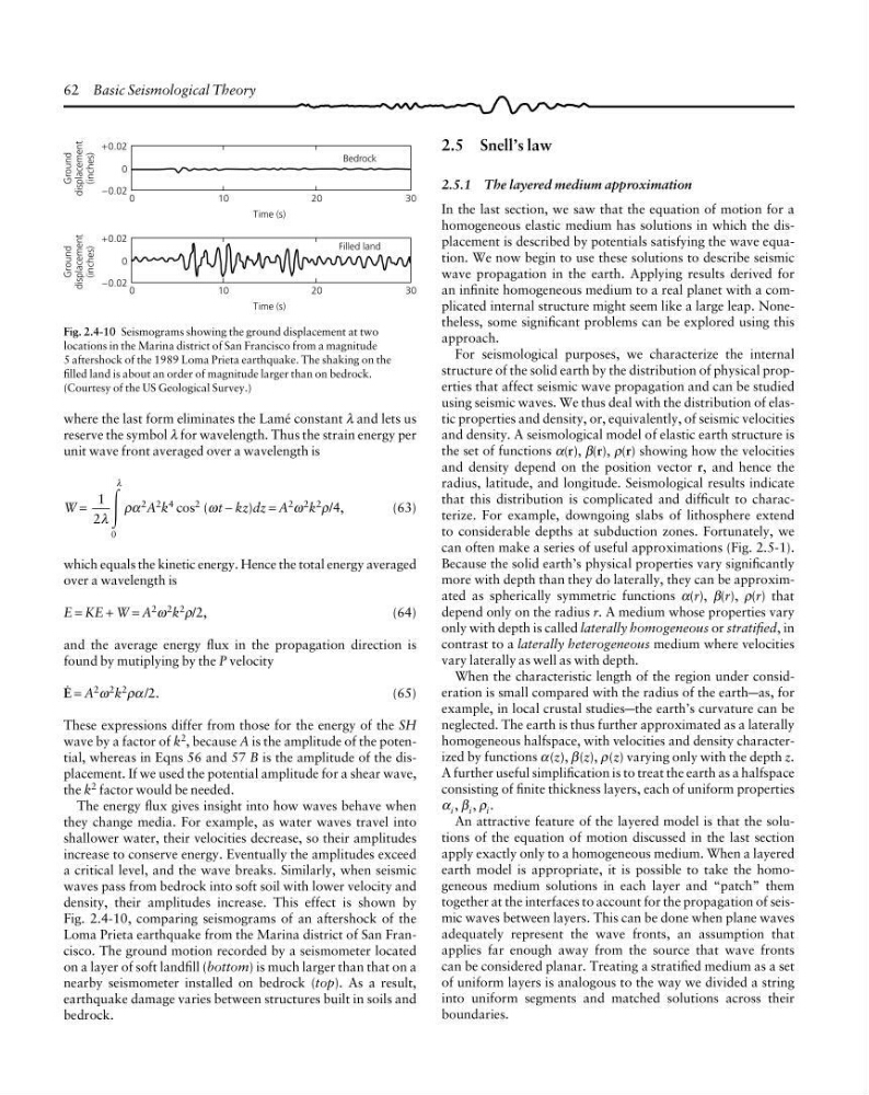
Fig. 2.4-10 Seismograms showing the ground displacement at two
locations in the Marina district of San Francisco from a magnitude
5 aftershock of the 1989 Loma Prieta earthquake. The shaking on the
filled land is about an order of magnitude larger than on bedrock.
(Courtesy of the US Geological Survey.)
where the last form eliminates the Lamé constant λ and lets us
reserve the symbol λ for wavelength. Thus the strain energy per
unit wave front averaged over a wavelength is
W =
1
2
0
λ
λ
Ύ
ρα
2
A
2 k
4 cos
2 (ωt − kz)dz = A
2
ω
2 k
2
ρ/4,
(63)
which equals the kinetic energy. Hence the total energy averaged
over a wavelength is
E = KE + W = A 2 ω 2 k 2 ρ/2,
(64)
and the average energy flux in the propagation direction is
found by mutiplying by the P velocity
0 = A 2 ω 2 k 2 ρα /2.
(65)
These expressions differ from those for the energy of the SH
wave by a factor of k 2 , because A is the amplitude of the potential, whereas in Eqns 56 and 57 B is the amplitude of the displacement. If we used the potential amplitude for a shear wave,
the k 2 factor would be needed.
The energy flux gives insight into how waves behave when
they change media. For example, as water waves travel into
shallower water, their velocities decrease, so their amplitudes
increase to conserve energy. Eventually the amplitudes exceed
a critical level, and the wave breaks. Similarly, when seismic
waves pass from bedrock into soft soil with lower velocity and
density, their amplitudes increase. This effect is shown by
Fig. 2.4-10, comparing seismograms of an aftershock of the
Loma Prieta earthquake from the Marina district of San Francisco. The ground motion recorded by a seismometer located
on a layer of soft landfill (bottom) is much larger than that on a
nearby seismometer installed on bedrock (top). As a result,
earthquake damage varies between structures built in soils and
bedrock.
2.5 Snell’s law
2.5.1 The layered medium approximation
In the last section, we saw that the equation of motion for a
homogeneous elastic medium has solutions in which the displacement is described by potentials satisfying the wave equation. We now begin to use these solutions to describe seismic
wave propagation in the earth. Applying results derived for
an infinite homogeneous medium to a real planet with a complicated internal structure might seem like a large leap. Nonetheless, some significant problems can be explored using this
approach.
For seismological purposes, we characterize the internal
structure of the solid earth by the distribution of physical properties that affect seismic wave propagation and can be studied
using seismic waves. We thus deal with the distribution of elastic properties and density, or, equivalently, of seismic velocities
and density. A seismological model of elastic earth structure is
the set of functions α(r), β(r), ρ(r) showing how the velocities
and density depend on the position vector r, and hence the
radius, latitude, and longitude. Seismological results indicate
that this distribution is complicated and difficult to characterize. For example, downgoing slabs of lithosphere extend
to considerable depths at subduction zones. Fortunately, we
can often make a series of useful approximations (Fig. 2.5-1).
Because the solid earth’s physical properties vary significantly
more with depth than they do laterally, they can be approximated as spherically symmetric functions α(r), β(r), ρ(r) that
depend only on the radius r. A medium whose properties vary
only with depth is called laterally homogeneous or stratified, in
contrast to a laterally heterogeneous medium where velocities
vary laterally as well as with depth.
When the characteristic length of the region under consideration is small compared with the radius of the earth—as, for
example, in local crustal studies—the earth’s curvature can be
neglected. The earth is thus further approximated as a laterally
homogeneous halfspace, with velocities and density characterized by functions α(z), β(z), ρ(z) varying only with the depth z.
A further useful simplification is to treat the earth as a halfspace
consisting of finite thickness layers, each of uniform properties
α i , β i , ρ i .
An attractive feature of the layered model is that the solutions of the equation of motion discussed in the last section
apply exactly only to a homogeneous medium. When a layered
earth model is appropriate, it is possible to take the homogeneous medium solutions in each layer and “patch” them
together at the interfaces to account for the propagation of seismic waves between layers. This can be done when plane waves
adequately represent the wave fronts, an assumption that
applies far enough away from the source that wave fronts
can be considered planar. Treating a stratified medium as a set
of uniform layers is analogous to the way we divided a string
into uniform segments and matched solutions across their
boundaries.
Ground
displacement
(inches)
+0.02
−0.02
0
1 0
2 0
3 0
Time (s)
0
Ground
displacement
(inches)
+0.02
−0.02
0
1 0
2 0
3 0
Time (s)
0
Filled land
Bedrock
Fig. 2.4-10 Seismograms showing the ground displacement at two
locations in the Marina district of San Francisco from a magnitude
5 aftershock of the 1989 Loma Prieta earthquake. The shaking on the
filled land is about an order of magnitude larger than on bedrock.
(Courtesy of the US Geological Survey.)
where the last form eliminates the Lamé constant λ and lets us
reserve the symbol λ for wavelength. Thus the strain energy per
unit wave front averaged over a wavelength is
W =
1
2
0
λ
λ
Ύ
ρα
2
A
2 k
4 cos
2 (ωt − kz)dz = A
2
ω
2 k
2
ρ/4,
(63)
which equals the kinetic energy. Hence the total energy averaged
over a wavelength is
E = KE + W = A 2 ω 2 k 2 ρ/2,
(64)
and the average energy flux in the propagation direction is
found by mutiplying by the P velocity
0 = A 2 ω 2 k 2 ρα /2.
(65)
These expressions differ from those for the energy of the SH
wave by a factor of k 2 , because A is the amplitude of the potential, whereas in Eqns 56 and 57 B is the amplitude of the displacement. If we used the potential amplitude for a shear wave,
the k 2 factor would be needed.
The energy flux gives insight into how waves behave when
they change media. For example, as water waves travel into
shallower water, their velocities decrease, so their amplitudes
increase to conserve energy. Eventually the amplitudes exceed
a critical level, and the wave breaks. Similarly, when seismic
waves pass from bedrock into soft soil with lower velocity and
density, their amplitudes increase. This effect is shown by
Fig. 2.4-10, comparing seismograms of an aftershock of the
Loma Prieta earthquake from the Marina district of San Francisco. The ground motion recorded by a seismometer located
on a layer of soft landfill (bottom) is much larger than that on a
nearby seismometer installed on bedrock (top). As a result,
earthquake damage varies between structures built in soils and
bedrock.