

when compressed. 6 In an ideal fluid, K = λ, so in this case λ has
an easy physical interpretation.
Writing the constitutive equation (70) in terms of K and µ,
σ ij = Kθδ ij + 2µ(e ij − θδ ij /3)
(75)
shows that the response to an applied stress has two parts: a
volume change characterized by K and a shear deformation,
or change in shape, characterized by µ.
Two other elastic constants are defined by pulling the material along only one axis, leading to a state of stress called
uniaxial tension. If the tension is applied along the x 1 axis, then
by Equation 70,
σ 11 = (λ + 2µ)e 11 + λe 22 + λe 33
σ 22 = 0 = λe 11 + (λ + 2µ)e 22 + λe 33
σ 33 = 0 = λe 11 + λe 22 + (λ + 2µ)e 33 .
(76)
Subtracting the last two equations shows that e 22 = e 33 , so
e
e
e
e
22
33
11
11
2 (
)
,
=
=
−
+
= −
λ
λ µ
ν
(77)
where ν, defined as Poisson’s ratio, gives the ratio of the contraction along the other two axes to the extension along the
axis where tension was applied. Substituting in the first line in
Eqn 76 yields
σ
µ λ
µ
λ µ
11
11
3
2
e
E
(
)
,
=
+
+
=
(78)
where E is called Young’s modulus, the ratio of the tensional
stress to the resulting extensional strain.
The elastic constants E, ν, and K are often used in engineering because they are easily measured by simple experiments.
However, for seismic wave propagation, λ, µ, and sometimes
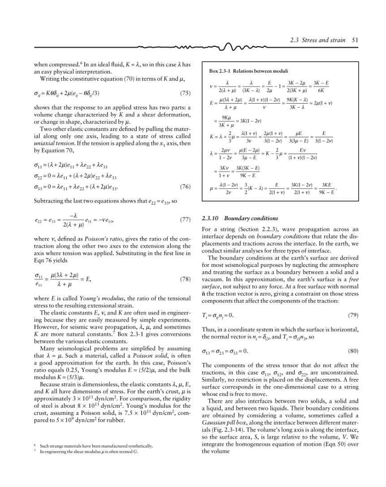
K are more natural constants. 7 Box 2.3-1 gives conversions
between the various elastic constants.
Many seismological problems are simplified by assuming
that λ = µ. Such a material, called a Poisson solid, is often
a good approximation for the earth. In this case, Poisson’s
ratio equals 0.25, Young’s modulus E = (5/2)µ, and the bulk
modulus K = (5/3)µ.
Because strain is dimensionless, the elastic constants λ, µ, E,
and K all have dimensions of stress. For the earth’s crust, µ is
approximately 3 × 10 11 dyn/cm 2 . For comparison, the rigidity
of steel is about 8 × 10 11 dyn/cm 2 . Young’s modulus for the
crust, assuming a Poisson solid, is 7.5 × 10
11 dyn/cm
2 , compared to 5 × 10 9 dyn/cm 2 for rubber.
Box 2.3-1 Relations between moduli
ν
λ
λ µ
λ
λ
µ
µ
µ
(
) (
)
(
)
=
+
=
−
=
− =
−
+
=
−
2
3
2
1
3
2
2 3
3
6
K
E
K
K
K E
K
E
K K
K
(
)
(
)(
)
(
)
(
)
=
+
+
=
+
−
=
−
−
=
+
µ λ
µ
λ µ
λ
ν
ν
ν
λ
λ
µ
ν
3
2
1
1 2
9
3
2 1
=
+
=
−
(
)
9
3
3 1 2
K
K
K
µ
µ
ν
K
E
E
E
(
)
(
)
(
)
(
)
(
)
= +
=
+ =
+
−
=
−
=
−
λ
µ
λ
ν
ν
µ
ν
ν
µ
µ
ν
2
3
1
3
2 1
3 1 2
3 3
3 1 2
λ
µν
ν
µ
µ
µ
µ
ν
ν
ν
(
)
(
)(
)
= −
=
−
−
= −
= +
−
2
1 2
2
3
2
3
1
1 2
E
E
K
E
= +
=
−
−
(
)
3
1
3 3
9
K
K K E
K E
ν
ν
µ
λ
ν
ν
λ
ν
ν
ν
(
)
(
)
(
)
(
)
(
)
.
=
−
=
− =
+
=
−
+
=
−
1 2
2
3
2
2 1
3 1 2
2 1
3
9
K
E
K
K E
K E
2.3.10 Boundary conditions
For a string (Section 2.2.3), wave propagation across an
interface depends on boundary conditions that relate the displacements and tractions across the interface. In the earth, we
conduct similar analyses for three types of interface.
The boundary conditions at the earth’s surface are derived
for most seismological purposes by neglecting the atmosphere
and treating the surface as a boundary between a solid and a
vacuum. In this approximation, the earth’s surface is a free
surface, not subject to any force. At a free surface with normal
4 the traction vector is zero, giving a constraint on those stress
components that affect the components of the traction:
T i = σ ij n j = 0.
(79)
Thus, in a coordinate system in which the surface is horizontal,
the normal vector is n i = δ i3 , and T i = σ i3 n 3 , so
σ 13 = σ 23 = σ 33 = 0.
(80)
The components of the stress tensor that do not affect the
tractions, in this case σ 11 , σ 12 , and σ 22 , are unconstrained.
Similarly, no restriction is placed on the displacements. A free
surface corresponds in the one-dimensional case to a string
whose end is free to move.
There are also interfaces between two solids, a solid and
a liquid, and between two liquids. Their boundary conditions
are obtained by considering a volume, sometimes called a
Gaussian pill box, along the interface between different materials (Fig. 2.3-14). The volume’s long axis is along the interface,
so the surface area, S, is large relative to the volume, V. We
integrate the homogeneous equation of motion (Eqn 50) over
the volume
2.3 Stress and strain 51
6 Such strange materials have been manufactured synthetically.
7 In engineering the shear modulus µ is often termed G.
an easy physical interpretation.
Writing the constitutive equation (70) in terms of K and µ,
σ ij = Kθδ ij + 2µ(e ij − θδ ij /3)
(75)
shows that the response to an applied stress has two parts: a
volume change characterized by K and a shear deformation,
or change in shape, characterized by µ.
Two other elastic constants are defined by pulling the material along only one axis, leading to a state of stress called
uniaxial tension. If the tension is applied along the x 1 axis, then
by Equation 70,
σ 11 = (λ + 2µ)e 11 + λe 22 + λe 33
σ 22 = 0 = λe 11 + (λ + 2µ)e 22 + λe 33
σ 33 = 0 = λe 11 + λe 22 + (λ + 2µ)e 33 .
(76)
Subtracting the last two equations shows that e 22 = e 33 , so
e
e
e
e
22
33
11
11
2 (
)
,
=
=
−
+
= −
λ
λ µ
ν
(77)
where ν, defined as Poisson’s ratio, gives the ratio of the contraction along the other two axes to the extension along the
axis where tension was applied. Substituting in the first line in
Eqn 76 yields
σ
µ λ
µ
λ µ
11
11
3
2
e
E
(
)
,
=
+
+
=
(78)
where E is called Young’s modulus, the ratio of the tensional
stress to the resulting extensional strain.
The elastic constants E, ν, and K are often used in engineering because they are easily measured by simple experiments.
However, for seismic wave propagation, λ, µ, and sometimes
K are more natural constants. 7 Box 2.3-1 gives conversions
between the various elastic constants.
Many seismological problems are simplified by assuming
that λ = µ. Such a material, called a Poisson solid, is often
a good approximation for the earth. In this case, Poisson’s
ratio equals 0.25, Young’s modulus E = (5/2)µ, and the bulk
modulus K = (5/3)µ.
Because strain is dimensionless, the elastic constants λ, µ, E,
and K all have dimensions of stress. For the earth’s crust, µ is
approximately 3 × 10 11 dyn/cm 2 . For comparison, the rigidity
of steel is about 8 × 10 11 dyn/cm 2 . Young’s modulus for the
crust, assuming a Poisson solid, is 7.5 × 10
11 dyn/cm
2 , compared to 5 × 10 9 dyn/cm 2 for rubber.
Box 2.3-1 Relations between moduli
ν
λ
λ µ
λ
λ
µ
µ
µ
(
) (
)
(
)
=
+
=
−
=
− =
−
+
=
−
2
3
2
1
3
2
2 3
3
6
K
E
K
K
K E
K
E
K K
K
(
)
(
)(
)
(
)
(
)
=
+
+
=
+
−
=
−
−
=
+
µ λ
µ
λ µ
λ
ν
ν
ν
λ
λ
µ
ν
3
2
1
1 2
9
3
2 1
=
+
=
−
(
)
9
3
3 1 2
K
K
K
µ
µ
ν
K
E
E
E
(
)
(
)
(
)
(
)
(
)
= +
=
+ =
+
−
=
−
=
−
λ
µ
λ
ν
ν
µ
ν
ν
µ
µ
ν
2
3
1
3
2 1
3 1 2
3 3
3 1 2
λ
µν
ν
µ
µ
µ
µ
ν
ν
ν
(
)
(
)(
)
= −
=
−
−
= −
= +
−
2
1 2
2
3
2
3
1
1 2
E
E
K
E
= +
=
−
−
(
)
3
1
3 3
9
K
K K E
K E
ν
ν
µ
λ
ν
ν
λ
ν
ν
ν
(
)
(
)
(
)
(
)
(
)
.
=
−
=
− =
+
=
−
+
=
−
1 2
2
3
2
2 1
3 1 2
2 1
3
9
K
E
K
K E
K E
2.3.10 Boundary conditions
For a string (Section 2.2.3), wave propagation across an
interface depends on boundary conditions that relate the displacements and tractions across the interface. In the earth, we
conduct similar analyses for three types of interface.
The boundary conditions at the earth’s surface are derived
for most seismological purposes by neglecting the atmosphere
and treating the surface as a boundary between a solid and a
vacuum. In this approximation, the earth’s surface is a free
surface, not subject to any force. At a free surface with normal
4 the traction vector is zero, giving a constraint on those stress
components that affect the components of the traction:
T i = σ ij n j = 0.
(79)
Thus, in a coordinate system in which the surface is horizontal,
the normal vector is n i = δ i3 , and T i = σ i3 n 3 , so
σ 13 = σ 23 = σ 33 = 0.
(80)
The components of the stress tensor that do not affect the
tractions, in this case σ 11 , σ 12 , and σ 22 , are unconstrained.
Similarly, no restriction is placed on the displacements. A free
surface corresponds in the one-dimensional case to a string
whose end is free to move.
There are also interfaces between two solids, a solid and
a liquid, and between two liquids. Their boundary conditions
are obtained by considering a volume, sometimes called a
Gaussian pill box, along the interface between different materials (Fig. 2.3-14). The volume’s long axis is along the interface,
so the surface area, S, is large relative to the volume, V. We
integrate the homogeneous equation of motion (Eqn 50) over
the volume
2.3 Stress and strain 51
6 Such strange materials have been manufactured synthetically.
7 In engineering the shear modulus µ is often termed G.