

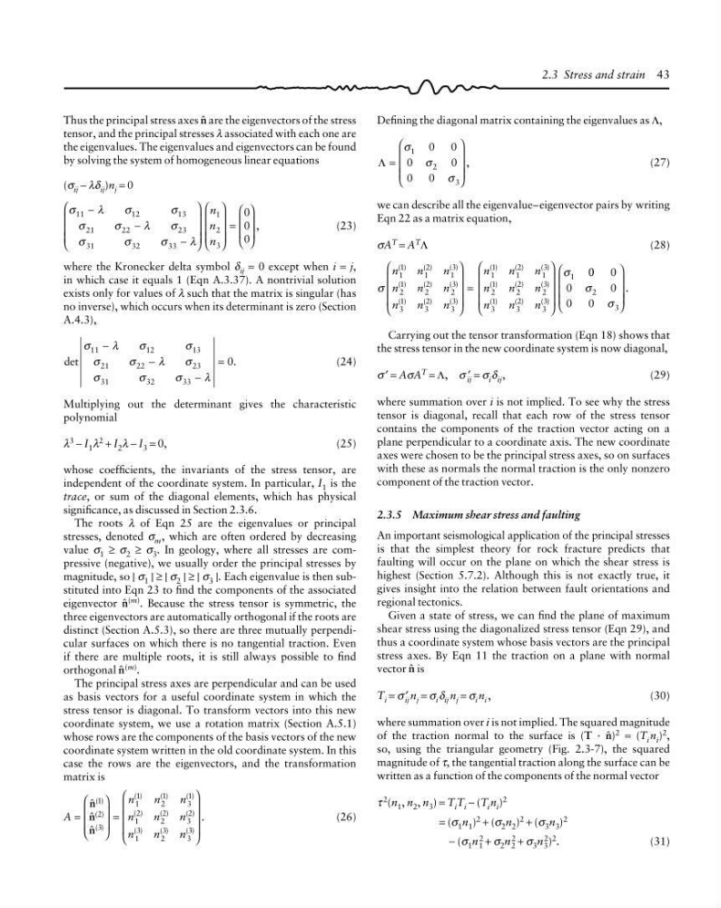
Thus the principal stress axes 4 are the eigenvectors of the stress
tensor, and the principal stresses λ associated with each one are
the eigenvalues. The eigenvalues and eigenvectors can be found
by solving the system of homogeneous linear equations
(σ ij − λδ ij )n j = 0
σ
λ
σ
σ
σ
σ
λ
σ
σ
σ
σ
λ
11
12
13
21
22
23
31
32
33
1
2
3
0
0
0
,
−
−
−
⎛
⎝
⎜
⎜
⎜
⎞
⎠
⎟
⎟
⎟
⎛
⎝
⎜
⎜
⎜
⎞
⎠
⎟
⎟
⎟
=
⎛
⎝
⎜
⎜
⎞
⎠
⎟
⎟
n
n
n
(23)
where the Kronecker delta symbol δ ij = 0 except when i = j,
in which case it equals 1 (Eqn A.3.37). A nontrivial solution
exists only for values of λ such that the matrix is singular (has
no inverse), which occurs when its determinant is zero (Section
A.4.3),
det
.
σ
λ
σ
σ
σ
σ
λ
σ
σ
σ
σ
λ
11
12
13
21
22
23
31
32
33
0
−
−
−
=
(24)
Multiplying out the determinant gives the characteristic
polynomial
λ
3
− I 1 λ
2
+ I 2 λ − I 3 = 0,
(25)
whose coefficients, the invariants of the stress tensor, are
independent of the coordinate system. In particular, I 1 is the
trace, or sum of the diagonal elements, which has physical
significance, as discussed in Section 2.3.6.
The roots λ of Eqn 25 are the eigenvalues or principal
stresses, denoted σ m , which are often ordered by decreasing
value σ 1 ≥ σ 2 ≥ σ 3 . In geology, where all stresses are compressive (negative), we usually order the principal stresses by
magnitude, so | σ 1 | ≥ | σ 2 | ≥ | σ 3 |. Each eigenvalue is then substituted into Eqn 23 to find the components of the associated
eigenvector 4 (m) . Because the stress tensor is symmetric, the
three eigenvectors are automatically orthogonal if the roots are
distinct (Section A.5.3), so there are three mutually perpendicular surfaces on which there is no tangential traction. Even
if there are multiple roots, it is still always possible to find
orthogonal 4
(m)
.
The principal stress axes are perpendicular and can be used
as basis vectors for a useful coordinate system in which the
stress tensor is diagonal. To transform vectors into this new
coordinate system, we use a rotation matrix (Section A.5.1)
whose rows are the components of the basis vectors of the new
coordinate system written in the old coordinate system. In this
case the rows are the eigenvectors, and the transformation
matrix is
A
n
n
n
n
n
n
n
n
n
.
( )
( )
( )
( )
( )
( )
( )
( )
( )
( )
( )
( )
=
⎛
⎝
⎜
⎜
⎞
⎠
⎟
⎟
=
⎛
⎝
⎜
⎜
⎜
⎞
⎠
⎟
⎟
⎟
4
4
4
1
2
3
1
1
2
1
3
1
1
2
2
2
3
2
1
3
2
3
3
3
(26)
2.3 Stress and strain 43
Defining the diagonal matrix containing the eigenvalues as Λ,
Λ
,
=
⎛
⎝
⎜
⎜
⎜
⎞
⎠
⎟
⎟
⎟
σ
σ
σ
1
2
3
0 0
0
0
0 0
(27)
we can describe all the eigenvalue–eigenvector pairs by writing
Eqn 22 as a matrix equation,
σA T = A T Λ
(28)
σ
σ
n
n
n
n
n
n
n
n
n
n
n
n
n
n
n
n
n
n
1
1
1
2
1
3
2
1
2
2
2
3
3
1
3
2
3
3
1
1
1
2
1
3
2
1
2
2
2
3
3
1
3
2
3
3
1
( )
( )
( )
( )
( )
( )
( )
( )
( )
( )
( )
( )
( )
( )
( )
( )
( )
( )
⎛
⎝
⎜
⎜
⎜
⎞
⎠
⎟
⎟
⎟
=
⎛
⎝
⎜
⎜
⎜
⎞
⎠
⎟
⎟
⎟
0 0 0
0
0
0 0
2
3
σ
σ
⎛
⎝
⎜
⎜
⎜
⎞
⎠
⎟
⎟
⎟
.
Carrying out the tensor transformation (Eqn 18) shows that
the stress tensor in the new coordinate system is now diagonal,
σ ′ = AσA T = Λ, σ ′
ij = σ i δ ij ,
(29)
where summation over i is not implied. To see why the stress
tensor is diagonal, recall that each row of the stress tensor
contains the components of the traction vector acting on a
plane perpendicular to a coordinate axis. The new coordinate
axes were chosen to be the principal stress axes, so on surfaces
with these as normals the normal traction is the only nonzero
component of the traction vector.
2.3.5 Maximum shear stress and faulting
An important seismological application of the principal stresses
is that the simplest theory for rock fracture predicts that
faulting will occur on the plane on which the shear stress is
highest (Section 5.7.2). Although this is not exactly true, it
gives insight into the relation between fault orientations and
regional tectonics.
Given a state of stress, we can find the plane of maximum
shear stress using the diagonalized stress tensor (Eqn 29), and
thus a coordinate system whose basis vectors are the principal
stress axes. By Eqn 11 the traction on a plane with normal
vector 4 is
T i = σ ′
ij n j = σ i δ ij n j = σ i n i ,
(30)
where summation over i is not implied. The squared magnitude
of the traction normal to the surface is (T · 4) 2 = (T i n i ) 2 ,
so, using the triangular geometry (Fig. 2.3-7), the squared
magnitude of τ, the tangential traction along the surface can be
written as a function of the components of the normal vector
τ 2 (n 1 , n 2 , n 3 ) = T i T i − (T i n i ) 2
= (σ 1 n 1 ) 2 + (σ 2 n 2 ) 2 + (σ 3 n 3 ) 2
− (σ 1 n 2
1 + σ 2 n 2
2 + σ 3 n 2
3 ) 2 .
(31)
tensor, and the principal stresses λ associated with each one are
the eigenvalues. The eigenvalues and eigenvectors can be found
by solving the system of homogeneous linear equations
(σ ij − λδ ij )n j = 0
σ
λ
σ
σ
σ
σ
λ
σ
σ
σ
σ
λ
11
12
13
21
22
23
31
32
33
1
2
3
0
0
0
,
−
−
−
⎛
⎝
⎜
⎜
⎜
⎞
⎠
⎟
⎟
⎟
⎛
⎝
⎜
⎜
⎜
⎞
⎠
⎟
⎟
⎟
=
⎛
⎝
⎜
⎜
⎞
⎠
⎟
⎟
n
n
n
(23)
where the Kronecker delta symbol δ ij = 0 except when i = j,
in which case it equals 1 (Eqn A.3.37). A nontrivial solution
exists only for values of λ such that the matrix is singular (has
no inverse), which occurs when its determinant is zero (Section
A.4.3),
det
.
σ
λ
σ
σ
σ
σ
λ
σ
σ
σ
σ
λ
11
12
13
21
22
23
31
32
33
0
−
−
−
=
(24)
Multiplying out the determinant gives the characteristic
polynomial
λ
3
− I 1 λ
2
+ I 2 λ − I 3 = 0,
(25)
whose coefficients, the invariants of the stress tensor, are
independent of the coordinate system. In particular, I 1 is the
trace, or sum of the diagonal elements, which has physical
significance, as discussed in Section 2.3.6.
The roots λ of Eqn 25 are the eigenvalues or principal
stresses, denoted σ m , which are often ordered by decreasing
value σ 1 ≥ σ 2 ≥ σ 3 . In geology, where all stresses are compressive (negative), we usually order the principal stresses by
magnitude, so | σ 1 | ≥ | σ 2 | ≥ | σ 3 |. Each eigenvalue is then substituted into Eqn 23 to find the components of the associated
eigenvector 4 (m) . Because the stress tensor is symmetric, the
three eigenvectors are automatically orthogonal if the roots are
distinct (Section A.5.3), so there are three mutually perpendicular surfaces on which there is no tangential traction. Even
if there are multiple roots, it is still always possible to find
orthogonal 4
(m)
.
The principal stress axes are perpendicular and can be used
as basis vectors for a useful coordinate system in which the
stress tensor is diagonal. To transform vectors into this new
coordinate system, we use a rotation matrix (Section A.5.1)
whose rows are the components of the basis vectors of the new
coordinate system written in the old coordinate system. In this
case the rows are the eigenvectors, and the transformation
matrix is
A
n
n
n
n
n
n
n
n
n
.
( )
( )
( )
( )
( )
( )
( )
( )
( )
( )
( )
( )
=
⎛
⎝
⎜
⎜
⎞
⎠
⎟
⎟
=
⎛
⎝
⎜
⎜
⎜
⎞
⎠
⎟
⎟
⎟
4
4
4
1
2
3
1
1
2
1
3
1
1
2
2
2
3
2
1
3
2
3
3
3
(26)
2.3 Stress and strain 43
Defining the diagonal matrix containing the eigenvalues as Λ,
Λ
,
=
⎛
⎝
⎜
⎜
⎜
⎞
⎠
⎟
⎟
⎟
σ
σ
σ
1
2
3
0 0
0
0
0 0
(27)
we can describe all the eigenvalue–eigenvector pairs by writing
Eqn 22 as a matrix equation,
σA T = A T Λ
(28)
σ
σ
n
n
n
n
n
n
n
n
n
n
n
n
n
n
n
n
n
n
1
1
1
2
1
3
2
1
2
2
2
3
3
1
3
2
3
3
1
1
1
2
1
3
2
1
2
2
2
3
3
1
3
2
3
3
1
( )
( )
( )
( )
( )
( )
( )
( )
( )
( )
( )
( )
( )
( )
( )
( )
( )
( )
⎛
⎝
⎜
⎜
⎜
⎞
⎠
⎟
⎟
⎟
=
⎛
⎝
⎜
⎜
⎜
⎞
⎠
⎟
⎟
⎟
0 0 0
0
0
0 0
2
3
σ
σ
⎛
⎝
⎜
⎜
⎜
⎞
⎠
⎟
⎟
⎟
.
Carrying out the tensor transformation (Eqn 18) shows that
the stress tensor in the new coordinate system is now diagonal,
σ ′ = AσA T = Λ, σ ′
ij = σ i δ ij ,
(29)
where summation over i is not implied. To see why the stress
tensor is diagonal, recall that each row of the stress tensor
contains the components of the traction vector acting on a
plane perpendicular to a coordinate axis. The new coordinate
axes were chosen to be the principal stress axes, so on surfaces
with these as normals the normal traction is the only nonzero
component of the traction vector.
2.3.5 Maximum shear stress and faulting
An important seismological application of the principal stresses
is that the simplest theory for rock fracture predicts that
faulting will occur on the plane on which the shear stress is
highest (Section 5.7.2). Although this is not exactly true, it
gives insight into the relation between fault orientations and
regional tectonics.
Given a state of stress, we can find the plane of maximum
shear stress using the diagonalized stress tensor (Eqn 29), and
thus a coordinate system whose basis vectors are the principal
stress axes. By Eqn 11 the traction on a plane with normal
vector 4 is
T i = σ ′
ij n j = σ i δ ij n j = σ i n i ,
(30)
where summation over i is not implied. The squared magnitude
of the traction normal to the surface is (T · 4) 2 = (T i n i ) 2 ,
so, using the triangular geometry (Fig. 2.3-7), the squared
magnitude of τ, the tangential traction along the surface can be
written as a function of the components of the normal vector
τ 2 (n 1 , n 2 , n 3 ) = T i T i − (T i n i ) 2
= (σ 1 n 1 ) 2 + (σ 2 n 2 ) 2 + (σ 3 n 3 ) 2
− (σ 1 n 2
1 + σ 2 n 2
2 + σ 3 n 2
3 ) 2 .
(31)