

462 Appendix
r
Equator
(0°, 0°)
x 1
φ
θ
e θ
eφ
e r
x 3
North pole
(0°, 90°)
x 2
ˆ
ˆ
ˆ
0.2
1.2
1.0
0.8
0.6
0.4
0
1.0
0.8
0.6
0.4
Fig. A.6-5 Top: streamlines showing
the velocity of fluid flow around an
object. Numbers on streamlines show the
magnitude of the velocity. Bottom: contours
of the curl for this velocity field. The curl is
greatest near the sphere, where the fluid flow
lines are the most curved. (After Batchelor,
1967. Reprinted with the permission of
Cambridge University Press.)
an obscure-looking relation that is useful in deriving the existence of P and S waves.
A.7 Spherical coordinates
The vector operations discussed so far were performed in
Cartesian coordinates, in which the unit basis vectors (ê 1 , ê 2 , ê 3 )
point in the same direction everywhere. There are, however,
situations in which non-Cartesian coordinate systems without
these nice properties are useful. In particular, spherical coordinates often simplify the solution of problems with a high degree
of symmetry about a point.
A.7.1 The spherical coordinate system
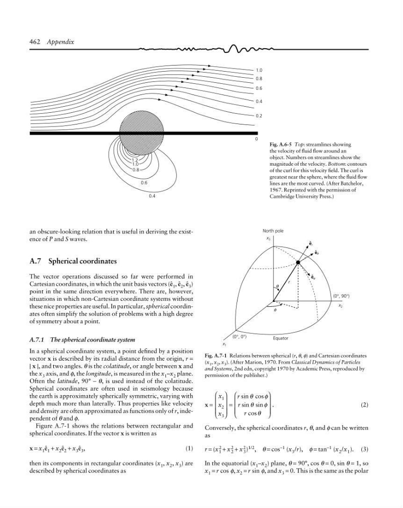
In a spherical coordinate system, a point defined by a position
vector x is described by its radial distance from the origin, r =
| x |, and two angles. θ is the colatitude, or angle between x and
the x 3 axis, and φ, the longitude, is measured in the x 1 –x 2 plane.
Often the latitude, 90° − θ, is used instead of the colatitude.
Spherical coordinates are often used in seismology because
the earth is approximately spherically symmetric, varying with
depth much more than laterally. Thus properties like velocity
and density are often approximated as functions only of r, independent of θ and φ.
Figure A.7-1 shows the relations between rectangular and
spherical coordinates. If the vector x is written as
x = x 1 ê 1 + x 2 ê 2 + x 3 ê 3 ,
(1)
then its components in rectangular coordinates (x 1 , x 2 , x 3 ) are
described by spherical coordinates as
Fig. A.7-1 Relations between spherical (r, θ, φ) and Cartesian coordinates
(x 1 , x 2 , x 3 ). (After Marion, 1970. From Classical Dynamics of Particles
and Systems, 2nd edn, copyright 1970 by Academic Press, reproduced by
permission of the publisher.)
x =
x
x
x
r
r
r
1
2
3
⎛
⎝
⎜
⎜
⎜
⎞
⎠
⎟
⎟
⎟
=
⎛
⎝
⎜
⎜
⎜
⎞
⎠
⎟
⎟
⎟
sin cos
sin sin
cos
.
θ
φ
θ
φ
θ
(2)
Conversely, the spherical coordinates r, θ, and φ can be written
as
r = (x 2
1 + x 2
2 + x 2
3 ) 1/2 , θ = cos −1 (x 3 /r), φ = tan −1 (x 2 /x 1 ). (3)
In the equatorial (x 1 –x 2 ) plane, θ = 90°, cos θ = 0, sin θ = 1, so
x 1 = r cos φ, x 2 = r sin φ, and x 3 = 0. This is the same as the polar
r
Equator
(0°, 0°)
x 1
φ
θ
e θ
eφ
e r
x 3
North pole
(0°, 90°)
x 2
ˆ
ˆ
ˆ
0.2
1.2
1.0
0.8
0.6
0.4
0
1.0
0.8
0.6
0.4
Fig. A.6-5 Top: streamlines showing
the velocity of fluid flow around an
object. Numbers on streamlines show the
magnitude of the velocity. Bottom: contours
of the curl for this velocity field. The curl is
greatest near the sphere, where the fluid flow
lines are the most curved. (After Batchelor,
1967. Reprinted with the permission of
Cambridge University Press.)
an obscure-looking relation that is useful in deriving the existence of P and S waves.
A.7 Spherical coordinates
The vector operations discussed so far were performed in
Cartesian coordinates, in which the unit basis vectors (ê 1 , ê 2 , ê 3 )
point in the same direction everywhere. There are, however,
situations in which non-Cartesian coordinate systems without
these nice properties are useful. In particular, spherical coordinates often simplify the solution of problems with a high degree
of symmetry about a point.
A.7.1 The spherical coordinate system
In a spherical coordinate system, a point defined by a position
vector x is described by its radial distance from the origin, r =
| x |, and two angles. θ is the colatitude, or angle between x and
the x 3 axis, and φ, the longitude, is measured in the x 1 –x 2 plane.
Often the latitude, 90° − θ, is used instead of the colatitude.
Spherical coordinates are often used in seismology because
the earth is approximately spherically symmetric, varying with
depth much more than laterally. Thus properties like velocity
and density are often approximated as functions only of r, independent of θ and φ.
Figure A.7-1 shows the relations between rectangular and
spherical coordinates. If the vector x is written as
x = x 1 ê 1 + x 2 ê 2 + x 3 ê 3 ,
(1)
then its components in rectangular coordinates (x 1 , x 2 , x 3 ) are
described by spherical coordinates as
Fig. A.7-1 Relations between spherical (r, θ, φ) and Cartesian coordinates
(x 1 , x 2 , x 3 ). (After Marion, 1970. From Classical Dynamics of Particles
and Systems, 2nd edn, copyright 1970 by Academic Press, reproduced by
permission of the publisher.)
x =
x
x
x
r
r
r
1
2
3
⎛
⎝
⎜
⎜
⎜
⎞
⎠
⎟
⎟
⎟
=
⎛
⎝
⎜
⎜
⎜
⎞
⎠
⎟
⎟
⎟
sin cos
sin sin
cos
.
θ
φ
θ
φ
θ
(2)
Conversely, the spherical coordinates r, θ, and φ can be written
as
r = (x 2
1 + x 2
2 + x 2
3 ) 1/2 , θ = cos −1 (x 3 /r), φ = tan −1 (x 2 /x 1 ). (3)
In the equatorial (x 1 –x 2 ) plane, θ = 90°, cos θ = 0, sin θ = 1, so
x 1 = r cos φ, x 2 = r sin φ, and x 3 = 0. This is the same as the polar