

u(x) = u(x 1 , x 2 , x 3 )
= u 1 (x 1 , x 2 , x 3 )ê 1 + u 2 (x 1 , x 2 , x 3 )ê 2 + u 3 (x 1 , x 2 , x 3 )ê 3
(1)
as a function of position, and result in turn from forces derived
from spatial derivatives of the stress tensor.
Spatial variations of scalar, vector, or tensor fields are described using the vector differential operator “del”, ∇
∇ ∇
∇ ∇,
∇ ∇
,
,
.
=
⎛
⎝
⎜
⎞
⎠
⎟
ê
ê
ê
1
1
2
2
3
3
∂
∂
∂
∂
∂
∂
x
x
x
(2)
This operator has the form of a vector, but has meaning only
when applied to a scalar, vector, or tensor field. We first review
uses of the ∇
∇ ∇
∇ ∇ operator in Cartesian coordinates, and in the
next section discuss the more complicated forms for spherical
coordinates.
A.6.2 Gradient
The simplest application of the ∇
∇ ∇
∇ ∇ operator is the gradient,
a vector field formed from the spatial derivatives of a scalar
field. If φ(x) is a scalar function of position, the gradient is
defined by
grad ( )
( )
( )
( )
( ) ,
φ
φ
φ
φ
φ
x
x
x ê
x ê
x ê
=
=
+
+
∇ ∇
∂
∂
∂
∂
∂
∂
x
x
x
1
1
2
2
3
3
(3)
where ∂φ(x)/ ∂x 1 is the partial derivative of φ(x 1 , x 2 , x 3 ) with
respect to x 1 , for x 2 and x 3 held constant. The gradient is a
vector field whose components equal the partial derivative with
respect to the corresponding coordinate.
Expressions like Eqns 1 and 3 can be written more compactly
if the dependences on position are not written explicitly, i.e.,
∇ ∇φ
φ
φ
φ .
=
+
+
∂
∂
∂
∂
∂
∂
x
x
x
1
1
2
2
3
3
ê
ê
ê
(4)
In this notation, it is implicit that φ, its derivatives, and hence
the gradient, vary with position.
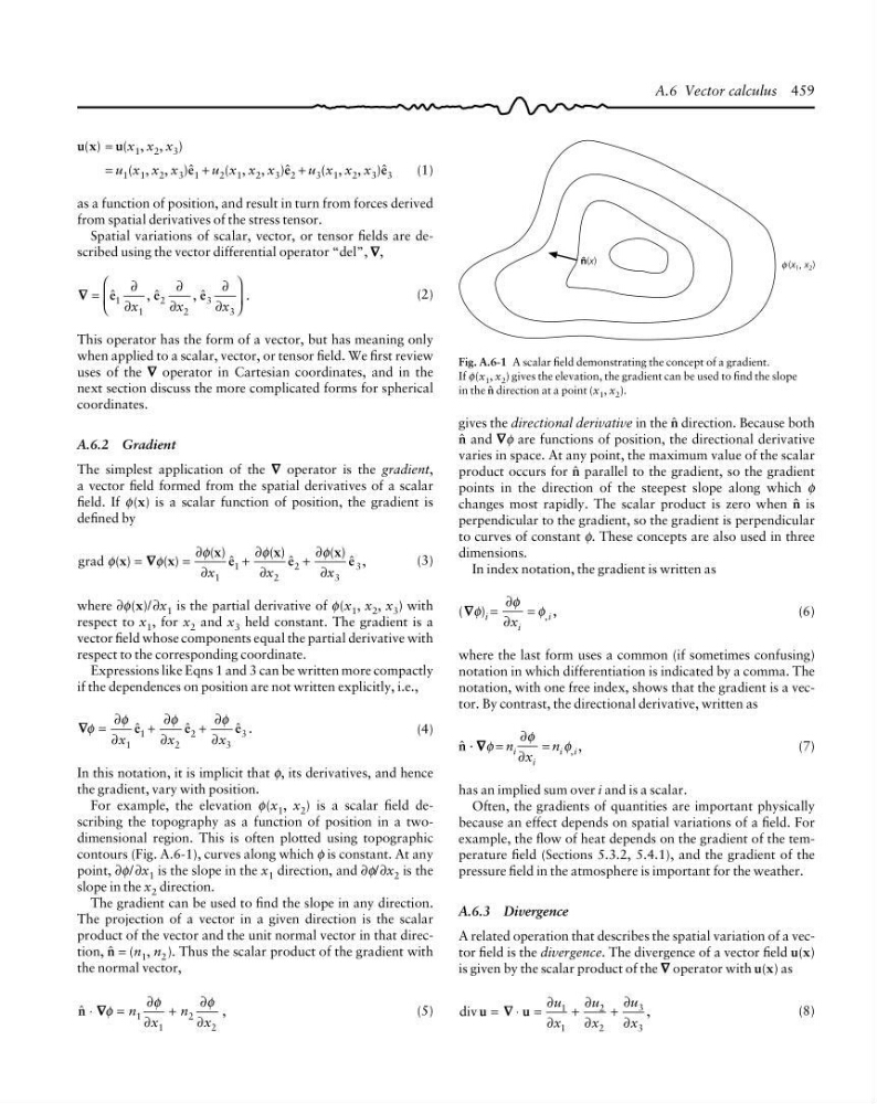
For example, the elevation φ(x 1 , x 2 ) is a scalar field describing the topography as a function of position in a twodimensional region. This is often plotted using topographic
contours (Fig. A.6-1), curves along which φ is constant. At any
point, ∂φ/ ∂x 1 is the slope in the x 1 direction, and ∂φ/ ∂x 2 is the
slope in the x 2 direction.
The gradient can be used to find the slope in any direction.
The projection of a vector in a given direction is the scalar
product of the vector and the unit normal vector in that direction, 4 = (n 1 , n 2 ). Thus the scalar product of the gradient with
the normal vector,
4
,
⋅
=
+
∇ ∇φ
φ
φ
n
x
n
x
1
1
2
2
∂
∂
∂
∂
(5)
Fig. A.6-1 A scalar field demonstrating the concept of a gradient.
If φ(x 1 , x 2 ) gives the elevation, the gradient can be used to find the slope
in the 4 direction at a point (x 1 , x 2 ).
ˆ
n(x)
(x 1 , x 2 )
φ
gives the directional derivative in the 4 direction. Because both
4 and ∇
∇ ∇
∇ ∇φ are functions of position, the directional derivative
varies in space. At any point, the maximum value of the scalar
product occurs for 4 parallel to the gradient, so the gradient
points in the direction of the steepest slope along which φ
changes most rapidly. The scalar product is zero when 4 is
perpendicular to the gradient, so the gradient is perpendicular
to curves of constant φ. These concepts are also used in three
dimensions.
In index notation, the gradient is written as
(∇ ∇ ∇
∇ ∇φ) i =
∂
∂
φ
x i
= φ , i ,
(6)
where the last form uses a common (if sometimes confusing)
notation in which differentiation is indicated by a comma. The
notation, with one free index, shows that the gradient is a vector. By contrast, the directional derivative, written as
4 · ∇
∇ ∇
∇ ∇φ = n i
∂
∂
φ
x i
= n i φ , i ,
(7)
has an implied sum over i and is a scalar.
Often, the gradients of quantities are important physically
because an effect depends on spatial variations of a field. For
example, the flow of heat depends on the gradient of the temperature field (Sections 5.3.2, 5.4.1), and the gradient of the
pressure field in the atmosphere is important for the weather.
A.6.3 Divergence
A related operation that describes the spatial variation of a vector field is the divergence. The divergence of a vector field u(x)
is given by the scalar product of the ∇
∇ ∇
∇ ∇ operator with u(x) as
div u
u
,
= ⋅ =
+
+
∇ ∇
∂
∂
∂
∂
∂
∂
u
x
u
x
u
x
1
1
2
2
3
3
(8)
A.6 Vector calculus 459
= u 1 (x 1 , x 2 , x 3 )ê 1 + u 2 (x 1 , x 2 , x 3 )ê 2 + u 3 (x 1 , x 2 , x 3 )ê 3
(1)
as a function of position, and result in turn from forces derived
from spatial derivatives of the stress tensor.
Spatial variations of scalar, vector, or tensor fields are described using the vector differential operator “del”, ∇
∇ ∇
∇ ∇,
∇ ∇
,
,
.
=
⎛
⎝
⎜
⎞
⎠
⎟
ê
ê
ê
1
1
2
2
3
3
∂
∂
∂
∂
∂
∂
x
x
x
(2)
This operator has the form of a vector, but has meaning only
when applied to a scalar, vector, or tensor field. We first review
uses of the ∇
∇ ∇
∇ ∇ operator in Cartesian coordinates, and in the
next section discuss the more complicated forms for spherical
coordinates.
A.6.2 Gradient
The simplest application of the ∇
∇ ∇
∇ ∇ operator is the gradient,
a vector field formed from the spatial derivatives of a scalar
field. If φ(x) is a scalar function of position, the gradient is
defined by
grad ( )
( )
( )
( )
( ) ,
φ
φ
φ
φ
φ
x
x
x ê
x ê
x ê
=
=
+
+
∇ ∇
∂
∂
∂
∂
∂
∂
x
x
x
1
1
2
2
3
3
(3)
where ∂φ(x)/ ∂x 1 is the partial derivative of φ(x 1 , x 2 , x 3 ) with
respect to x 1 , for x 2 and x 3 held constant. The gradient is a
vector field whose components equal the partial derivative with
respect to the corresponding coordinate.
Expressions like Eqns 1 and 3 can be written more compactly
if the dependences on position are not written explicitly, i.e.,
∇ ∇φ
φ
φ
φ .
=
+
+
∂
∂
∂
∂
∂
∂
x
x
x
1
1
2
2
3
3
ê
ê
ê
(4)
In this notation, it is implicit that φ, its derivatives, and hence
the gradient, vary with position.
For example, the elevation φ(x 1 , x 2 ) is a scalar field describing the topography as a function of position in a twodimensional region. This is often plotted using topographic
contours (Fig. A.6-1), curves along which φ is constant. At any
point, ∂φ/ ∂x 1 is the slope in the x 1 direction, and ∂φ/ ∂x 2 is the
slope in the x 2 direction.
The gradient can be used to find the slope in any direction.
The projection of a vector in a given direction is the scalar
product of the vector and the unit normal vector in that direction, 4 = (n 1 , n 2 ). Thus the scalar product of the gradient with
the normal vector,
4
,
⋅
=
+
∇ ∇φ
φ
φ
n
x
n
x
1
1
2
2
∂
∂
∂
∂
(5)
Fig. A.6-1 A scalar field demonstrating the concept of a gradient.
If φ(x 1 , x 2 ) gives the elevation, the gradient can be used to find the slope
in the 4 direction at a point (x 1 , x 2 ).
ˆ
n(x)
(x 1 , x 2 )
φ
gives the directional derivative in the 4 direction. Because both
4 and ∇
∇ ∇
∇ ∇φ are functions of position, the directional derivative
varies in space. At any point, the maximum value of the scalar
product occurs for 4 parallel to the gradient, so the gradient
points in the direction of the steepest slope along which φ
changes most rapidly. The scalar product is zero when 4 is
perpendicular to the gradient, so the gradient is perpendicular
to curves of constant φ. These concepts are also used in three
dimensions.
In index notation, the gradient is written as
(∇ ∇ ∇
∇ ∇φ) i =
∂
∂
φ
x i
= φ , i ,
(6)
where the last form uses a common (if sometimes confusing)
notation in which differentiation is indicated by a comma. The
notation, with one free index, shows that the gradient is a vector. By contrast, the directional derivative, written as
4 · ∇
∇ ∇
∇ ∇φ = n i
∂
∂
φ
x i
= n i φ , i ,
(7)
has an implied sum over i and is a scalar.
Often, the gradients of quantities are important physically
because an effect depends on spatial variations of a field. For
example, the flow of heat depends on the gradient of the temperature field (Sections 5.3.2, 5.4.1), and the gradient of the
pressure field in the atmosphere is important for the weather.
A.6.3 Divergence
A related operation that describes the spatial variation of a vector field is the divergence. The divergence of a vector field u(x)
is given by the scalar product of the ∇
∇ ∇
∇ ∇ operator with u(x) as
div u
u
,
= ⋅ =
+
+
∇ ∇
∂
∂
∂
∂
∂
∂
u
x
u
x
u
x
1
1
2
2
3
3
(8)
A.6 Vector calculus 459