

y = Ax
(16)
is also a vector in n dimensions. This is not the same as coordinate transformation; the vector x is transformed into
another distinct vector, with both vectors expressed in the same
coordinate system.
A physically important class of transformations convert a
vector into one parallel to the original vector, so that
Ax = λ x,
(17)
where A is a matrix, and λ is a scalar. The only effect of the
transformation is that the length of x changes by a factor of λ.
For a given A, it is useful to know which vectors x and scalars λ
satisfy this equation.
In three dimensions, the case most commonly encountered,
Eqn 17 can be written
(A − λI)x = 0
a
a
a
a
a
a
a
a
a
x
x
x
11
12
13
21
22
23
31
32
33
1
2
3
0
0
0
.
−
−
−
⎛
⎝
⎜
⎜
⎜
⎞
⎠
⎟
⎟
⎟
⎛
⎝
⎜
⎜
⎜
⎞
⎠
⎟
⎟
⎟
=
⎛
⎝
⎜
⎜
⎜
⎞
⎠
⎟
⎟
⎟
λ
λ
λ
(18)
This is a homogeneous system of linear equations, so nontrivial
solutions exist only if the matrix (A − λI) is singular. We thus
seek values of λ such that the determinant
|(
) | det
.
A
I
a
a
a
a
a
a
a
a
a
−
=
−
−
−
⎛
⎝
⎜
⎜
⎜
⎞
⎠
⎟
⎟
⎟
=
λ
λ
λ
λ
11
12
13
21
22
23
31
32
33
0
(19)
Evaluating the determinant gives the characteristic polynomial
λ 3 − I 1 λ 2 + I 2 λ − I 3 = 0,
(20)
which depends on three constants called the invariants of A:
I 1 = a 11 + a 22 + a 33 ,
I 2 = det
det
det
,
a
a
a
a
a
a
a
a
a
a
a
a
11
12
21
22
22
23
32
33
11
13
31
33
⎛
⎝
⎜
⎞
⎠
⎟ +
⎛
⎝
⎜
⎞
⎠
⎟ +
⎛
⎝
⎜
⎞
⎠
⎟
I 3 = det A.
(21)
I 1 , the first invariant, or trace, of A, is the sum of the diagonal
elements of A. The invariants of a matrix have significance for
stresses, strains, and earthquake moment tensors, because they
are not changed by orthogonal transformations.
The characteristic polynomial is a cubic equation in λ
with three roots, or eigenvalues, λ m for which the determinant
| A − λI | is zero. For each eigenvalue there is an associated nontrivial eigenvector, x (m) , satisfying
Ax (m) = λ m x (m) .
(22)
The components of the eigenvector, x 1
(m) , x 2
(m) , x 3
(m) , are found
by solving
a
a
a
a
a
a
a
a
a
x
x
x
m
m
m
m
m
m
11
12
13
21
22
23
31
32
33
1
2
3
0
0
0
.
( )
( )
( )
−
−
−
⎛
⎝
⎜
⎜
⎜
⎞
⎠
⎟
⎟
⎟
⎛
⎝
⎜
⎜
⎜
⎞
⎠
⎟
⎟
⎟
=
⎛
⎝
⎜
⎜
⎜
⎞
⎠
⎟
⎟
⎟
λ
λ
λ
(23)
Each eigenvalue and its associated eigenvector form a pair
satisfying Eqn 22. In general, an eigenvalue and the eigenvector associated with a different eigenvalue will not satisfy the
equation.
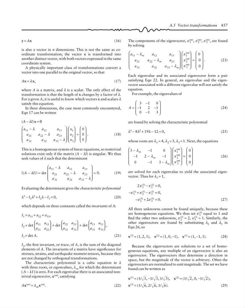
For example, the eigenvalues of
A =
−
−
−
−
⎛
⎝
⎜
⎜
⎞
⎠
⎟
⎟
3
1
0
1
2
1
0
1
3
(24)
are found by solving the characteristic polynomial
λ 3 − 8λ 2 + 19λ − 12 = 0,
(25)
whose roots are λ 1 = 4, λ 2 = 3, λ 3 = 1. Next, the equations
3
1
0
1
2
1
0
1
3
0
0
0
1
2
3
( )
( )
( )
−
−
−
−
−
−
−
⎛
⎝
⎜
⎜
⎜
⎞
⎠
⎟
⎟
⎟
⎛
⎝
⎜
⎜
⎜
⎞
⎠
⎟
⎟
⎟
=
⎛
⎝
⎜
⎜
⎜
⎞
⎠
⎟
⎟
⎟
λ
λ
λ
m
m
m
m
m
m
x
x
x
(26)
are solved for each eigenvalue to yield the associated eigenvector. Thus for λ 3 = 1,
2x 1
(3) − x 2
(3) = 0,
−x 1
(3) + x 2
(3) − x 3
(3) = 0,
−x 2
(3)
+ 2x 3
(3)
= 0.
(27)
All three unknowns cannot be found uniquely, because these
are homogeneous equations. We thus set x 1
(3) equal to 1 and
find the other two unknowns, x 2
(3)
= 2, x 3
(3)
= 1. Similarly, the
other eigenvectors are found by substituting λ 2 and λ 1 in
Eqn 26, so
x (3) = (1, 2, 1), x (2) = (1, 0, −1), x (1) = (1, −1, 1).
(28)
Because the eigenvectors are solutions to a set of homogeneous equations, any multiple of an eigenvector is also an
eigenvector. The eigenvectors thus determine a direction in
space, but the magnitude of the vector is arbitrary. Often the
eigenvectors are normalized to unit magnitude. The set we have
found can be written as
x (1) = (1/ 3, −1/ 3, 1/ 3), x (2) = (1/ 2 , 0, −1/ 2 ),
x (3) = (1/ 6, 2/ 6, 1/ 6).
(29)
A.5 Vector transformations 457
(16)
is also a vector in n dimensions. This is not the same as coordinate transformation; the vector x is transformed into
another distinct vector, with both vectors expressed in the same
coordinate system.
A physically important class of transformations convert a
vector into one parallel to the original vector, so that
Ax = λ x,
(17)
where A is a matrix, and λ is a scalar. The only effect of the
transformation is that the length of x changes by a factor of λ.
For a given A, it is useful to know which vectors x and scalars λ
satisfy this equation.
In three dimensions, the case most commonly encountered,
Eqn 17 can be written
(A − λI)x = 0
a
a
a
a
a
a
a
a
a
x
x
x
11
12
13
21
22
23
31
32
33
1
2
3
0
0
0
.
−
−
−
⎛
⎝
⎜
⎜
⎜
⎞
⎠
⎟
⎟
⎟
⎛
⎝
⎜
⎜
⎜
⎞
⎠
⎟
⎟
⎟
=
⎛
⎝
⎜
⎜
⎜
⎞
⎠
⎟
⎟
⎟
λ
λ
λ
(18)
This is a homogeneous system of linear equations, so nontrivial
solutions exist only if the matrix (A − λI) is singular. We thus
seek values of λ such that the determinant
|(
) | det
.
A
I
a
a
a
a
a
a
a
a
a
−
=
−
−
−
⎛
⎝
⎜
⎜
⎜
⎞
⎠
⎟
⎟
⎟
=
λ
λ
λ
λ
11
12
13
21
22
23
31
32
33
0
(19)
Evaluating the determinant gives the characteristic polynomial
λ 3 − I 1 λ 2 + I 2 λ − I 3 = 0,
(20)
which depends on three constants called the invariants of A:
I 1 = a 11 + a 22 + a 33 ,
I 2 = det
det
det
,
a
a
a
a
a
a
a
a
a
a
a
a
11
12
21
22
22
23
32
33
11
13
31
33
⎛
⎝
⎜
⎞
⎠
⎟ +
⎛
⎝
⎜
⎞
⎠
⎟ +
⎛
⎝
⎜
⎞
⎠
⎟
I 3 = det A.
(21)
I 1 , the first invariant, or trace, of A, is the sum of the diagonal
elements of A. The invariants of a matrix have significance for
stresses, strains, and earthquake moment tensors, because they
are not changed by orthogonal transformations.
The characteristic polynomial is a cubic equation in λ
with three roots, or eigenvalues, λ m for which the determinant
| A − λI | is zero. For each eigenvalue there is an associated nontrivial eigenvector, x (m) , satisfying
Ax (m) = λ m x (m) .
(22)
The components of the eigenvector, x 1
(m) , x 2
(m) , x 3
(m) , are found
by solving
a
a
a
a
a
a
a
a
a
x
x
x
m
m
m
m
m
m
11
12
13
21
22
23
31
32
33
1
2
3
0
0
0
.
( )
( )
( )
−
−
−
⎛
⎝
⎜
⎜
⎜
⎞
⎠
⎟
⎟
⎟
⎛
⎝
⎜
⎜
⎜
⎞
⎠
⎟
⎟
⎟
=
⎛
⎝
⎜
⎜
⎜
⎞
⎠
⎟
⎟
⎟
λ
λ
λ
(23)
Each eigenvalue and its associated eigenvector form a pair
satisfying Eqn 22. In general, an eigenvalue and the eigenvector associated with a different eigenvalue will not satisfy the
equation.
For example, the eigenvalues of
A =
−
−
−
−
⎛
⎝
⎜
⎜
⎞
⎠
⎟
⎟
3
1
0
1
2
1
0
1
3
(24)
are found by solving the characteristic polynomial
λ 3 − 8λ 2 + 19λ − 12 = 0,
(25)
whose roots are λ 1 = 4, λ 2 = 3, λ 3 = 1. Next, the equations
3
1
0
1
2
1
0
1
3
0
0
0
1
2
3
( )
( )
( )
−
−
−
−
−
−
−
⎛
⎝
⎜
⎜
⎜
⎞
⎠
⎟
⎟
⎟
⎛
⎝
⎜
⎜
⎜
⎞
⎠
⎟
⎟
⎟
=
⎛
⎝
⎜
⎜
⎜
⎞
⎠
⎟
⎟
⎟
λ
λ
λ
m
m
m
m
m
m
x
x
x
(26)
are solved for each eigenvalue to yield the associated eigenvector. Thus for λ 3 = 1,
2x 1
(3) − x 2
(3) = 0,
−x 1
(3) + x 2
(3) − x 3
(3) = 0,
−x 2
(3)
+ 2x 3
(3)
= 0.
(27)
All three unknowns cannot be found uniquely, because these
are homogeneous equations. We thus set x 1
(3) equal to 1 and
find the other two unknowns, x 2
(3)
= 2, x 3
(3)
= 1. Similarly, the
other eigenvectors are found by substituting λ 2 and λ 1 in
Eqn 26, so
x (3) = (1, 2, 1), x (2) = (1, 0, −1), x (1) = (1, −1, 1).
(28)
Because the eigenvectors are solutions to a set of homogeneous equations, any multiple of an eigenvector is also an
eigenvector. The eigenvectors thus determine a direction in
space, but the magnitude of the vector is arbitrary. Often the
eigenvectors are normalized to unit magnitude. The set we have
found can be written as
x (1) = (1/ 3, −1/ 3, 1/ 3), x (2) = (1/ 2 , 0, −1/ 2 ),
x (3) = (1/ 6, 2/ 6, 1/ 6).
(29)
A.5 Vector transformations 457