

Given the components u i in the unprimed system, the components u′ i in the primed system are found by taking the scalar
products of the vector with the basis vectors of the primed
system:
u′ 1 = ê′ 1 · u = (ê′ 1 · ê 1 )u 1 + (ê′ 1 · ê 2 )u 2 + (ê′ 1 · ê 3 )u 3
= a 11 u 1 + a 12 u 2 + a 13 u 3 ,
u′ 2 = ê′ 2 · u = a 21 u 1 + a 22 u 2 + a 23 u 3 ,
u′ 3 = ê′ 3 · u = a 31 u 1 + a 32 u 2 + a 33 u 3 .
(3)
These can be written as a matrix equation
u′ = Au, or
u
u
u
a
a
a
a
a
a
a
a
a
u
u
u
1
2
3
11
12
13
21
22
23
31
32
33
1
2
3
′
′
′
⎛
⎝
⎜
⎜
⎜
⎞
⎠
⎟
⎟
⎟
=
⎛
⎝
⎜
⎜
⎜
⎞
⎠
⎟
⎟
⎟
⎛
⎝
⎜
⎜
⎜
⎞
⎠
⎟
⎟
⎟
,
(4)
where A is the matrix that transforms a vector from the
unprimed to the primed system. Note that this is not a relation
between two different vectors u and u′ — it is a relationship
between the components of the same vector in two coordinate
systems. It turns out that the matrix A uniquely describes the
transformation between these coordinate systems.
For example, a unit basis vector for the unprimed system
ê 1 = 1ê 1 + 0ê 2 + 0ê 3 = (1, 0, 0)
(5)
has components in the primed system given by
a
a
a
a
a
a
a
a
a
a
a
a
11
21
31
11
12
13
21
22
23
31
32
33
1
0
0
⎛
⎝
⎜
⎜
⎜
⎞
⎠
⎟
⎟
⎟
=
⎛
⎝
⎜
⎜
⎜
⎞
⎠
⎟
⎟
⎟
⎛
⎝
⎜
⎜
⎜
⎞
⎠
⎟
⎟
⎟
,
(6)
and so is written
a 11 ê′ 1 + a 21 ê′ 2 + a 31 ê′ 3 = (a 11 , a 21 , a 31 )
(7)
in the primed system. The last expression is just the first column
of A. Similarly, the components of ê 2 and ê 3 in the primed
system are the second and third columns of A, respectively.
Thus the columns of the transformation matrix A are the basis
vectors of the unprimed system written in terms of their components in the primed system.
For example, consider rotating a Cartesian coordinate system by θ counterclockwise about the ê 3 axis, so that the only
rotation occurs in the ê 1 –ê 2 plane. The ê 3 axis is also the ê′ 3 axis
(Fig. A.5-2). The elements of the transformation matrix are
found by evaluating the scalar products of the basis vectors
a ij = ê′ i · ê j , so
a 11 = ê′ 1 · ê 1 = cos θ, a 12 = ê′ 1 · ê 2 = cos (90° − θ) = sin θ,
a 22 = ê′ 2 · ê 2 = cos θ, a 21 = ê′ 2 · ê 1 = cos (90° + θ) = −sin θ,
a 33 = ê′ 3 · ê 3 = 1,
a 13 = a 23 = a 31 = a 32 = 0,
(8)
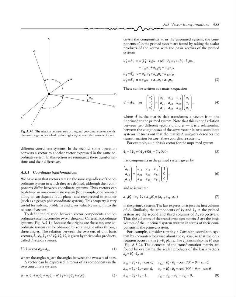
Fig. A.5-1 The relation between two orthogonal coordinate systems with
the same origin is described by the angles α ij between the two sets of axes.
α 32
α 12
x 1
x′ 1
x 2
x ′
2
α 22
x 3
x′ 3
u
A.5 Vector transformations 455
different coordinate systems. In the second, some operation
converts a vector to another vector expressed in the same coordinate system. In this section we summarize these transformations and their differences.
A.5.1 Coordinate transformations
We have seen that vectors remain the same regardless of the coordinate system in which they are defined, although their components differ between coordinate systems. Thus vectors can
be defined in one coordinate system (for example, one oriented
along an earthquake fault plane) and reexpressed in another
(such as a geographic coordinate system). This property is very
useful for solving problems and gives valuable insight into the
nature of vectors.
To define the relation between vector components and coordinate systems, consider two orthogonal Cartesian coordinate
systems (Fig. A.5-1). Because the origins are the same, one coordinate system can be obtained by rotating the other through
three angles. The relation between the two sets of unit basis
vectors, ê 1 , ê 2 , ê 3 and ê′ 1 , ê′ 2 , ê′ 3 , is given by their scalar products,
called direction cosines,
ê′ i · ê j = cos α ij = a ij ,
(1)
where the angles α ij are the angles between the two sets of axes.
A vector can be expressed in terms of its components in the
two coordinate systems
u = u 1 ê 1 + u 2 ê 2 + u 3 ê 3 = u′ 1 ê′ 1 + u′ 2 ê′ 2 + u′ 3 ê′ 3 .
(2)
products of the vector with the basis vectors of the primed
system:
u′ 1 = ê′ 1 · u = (ê′ 1 · ê 1 )u 1 + (ê′ 1 · ê 2 )u 2 + (ê′ 1 · ê 3 )u 3
= a 11 u 1 + a 12 u 2 + a 13 u 3 ,
u′ 2 = ê′ 2 · u = a 21 u 1 + a 22 u 2 + a 23 u 3 ,
u′ 3 = ê′ 3 · u = a 31 u 1 + a 32 u 2 + a 33 u 3 .
(3)
These can be written as a matrix equation
u′ = Au, or
u
u
u
a
a
a
a
a
a
a
a
a
u
u
u
1
2
3
11
12
13
21
22
23
31
32
33
1
2
3
′
′
′
⎛
⎝
⎜
⎜
⎜
⎞
⎠
⎟
⎟
⎟
=
⎛
⎝
⎜
⎜
⎜
⎞
⎠
⎟
⎟
⎟
⎛
⎝
⎜
⎜
⎜
⎞
⎠
⎟
⎟
⎟
,
(4)
where A is the matrix that transforms a vector from the
unprimed to the primed system. Note that this is not a relation
between two different vectors u and u′ — it is a relationship
between the components of the same vector in two coordinate
systems. It turns out that the matrix A uniquely describes the
transformation between these coordinate systems.
For example, a unit basis vector for the unprimed system
ê 1 = 1ê 1 + 0ê 2 + 0ê 3 = (1, 0, 0)
(5)
has components in the primed system given by
a
a
a
a
a
a
a
a
a
a
a
a
11
21
31
11
12
13
21
22
23
31
32
33
1
0
0
⎛
⎝
⎜
⎜
⎜
⎞
⎠
⎟
⎟
⎟
=
⎛
⎝
⎜
⎜
⎜
⎞
⎠
⎟
⎟
⎟
⎛
⎝
⎜
⎜
⎜
⎞
⎠
⎟
⎟
⎟
,
(6)
and so is written
a 11 ê′ 1 + a 21 ê′ 2 + a 31 ê′ 3 = (a 11 , a 21 , a 31 )
(7)
in the primed system. The last expression is just the first column
of A. Similarly, the components of ê 2 and ê 3 in the primed
system are the second and third columns of A, respectively.
Thus the columns of the transformation matrix A are the basis
vectors of the unprimed system written in terms of their components in the primed system.
For example, consider rotating a Cartesian coordinate system by θ counterclockwise about the ê 3 axis, so that the only
rotation occurs in the ê 1 –ê 2 plane. The ê 3 axis is also the ê′ 3 axis
(Fig. A.5-2). The elements of the transformation matrix are
found by evaluating the scalar products of the basis vectors
a ij = ê′ i · ê j , so
a 11 = ê′ 1 · ê 1 = cos θ, a 12 = ê′ 1 · ê 2 = cos (90° − θ) = sin θ,
a 22 = ê′ 2 · ê 2 = cos θ, a 21 = ê′ 2 · ê 1 = cos (90° + θ) = −sin θ,
a 33 = ê′ 3 · ê 3 = 1,
a 13 = a 23 = a 31 = a 32 = 0,
(8)
Fig. A.5-1 The relation between two orthogonal coordinate systems with
the same origin is described by the angles α ij between the two sets of axes.
α 32
α 12
x 1
x′ 1
x 2
x ′
2
α 22
x 3
x′ 3
u
A.5 Vector transformations 455
different coordinate systems. In the second, some operation
converts a vector to another vector expressed in the same coordinate system. In this section we summarize these transformations and their differences.
A.5.1 Coordinate transformations
We have seen that vectors remain the same regardless of the coordinate system in which they are defined, although their components differ between coordinate systems. Thus vectors can
be defined in one coordinate system (for example, one oriented
along an earthquake fault plane) and reexpressed in another
(such as a geographic coordinate system). This property is very
useful for solving problems and gives valuable insight into the
nature of vectors.
To define the relation between vector components and coordinate systems, consider two orthogonal Cartesian coordinate
systems (Fig. A.5-1). Because the origins are the same, one coordinate system can be obtained by rotating the other through
three angles. The relation between the two sets of unit basis
vectors, ê 1 , ê 2 , ê 3 and ê′ 1 , ê′ 2 , ê′ 3 , is given by their scalar products,
called direction cosines,
ê′ i · ê j = cos α ij = a ij ,
(1)
where the angles α ij are the angles between the two sets of axes.
A vector can be expressed in terms of its components in the
two coordinate systems
u = u 1 ê 1 + u 2 ê 2 + u 3 ê 3 = u′ 1 ê′ 1 + u′ 2 ê′ 2 + u′ 3 ê′ 3 .
(2)