

32 Basic Seismological Theory
which physical properties vary with depth, we need to treat
waves on a string with variable properties along its length.
The simplest situation is a string composed of segments with
uniform properties. If the segments are long enough, we treat
the displacement in each segment as composed of propagating waves described by the solution for a uniform string with
the appropriate properties, and then match solutions across the
boundaries between segments.
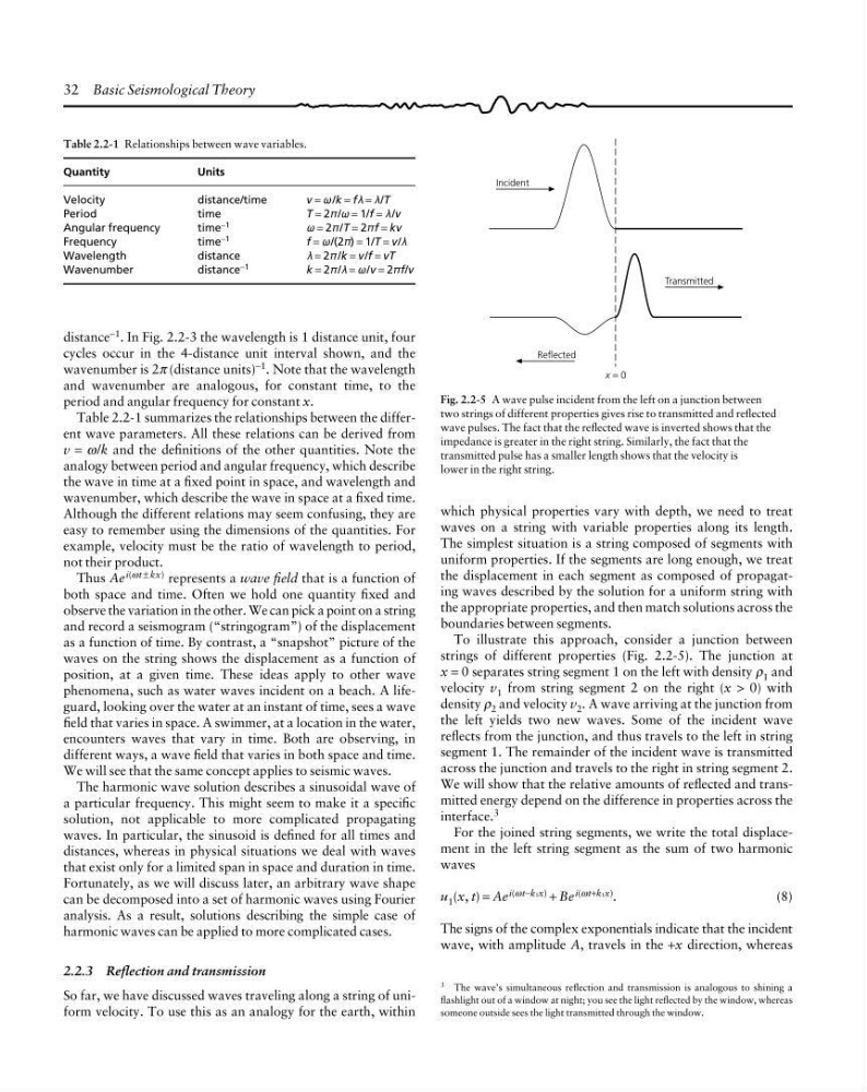
To illustrate this approach, consider a junction between
strings of different properties (Fig. 2.2-5). The junction at
x = 0 separates string segment 1 on the left with density ρ 1 and
velocity v 1 from string segment 2 on the right (x > 0) with
density ρ 2 and velocity v 2 . A wave arriving at the junction from
the left yields two new waves. Some of the incident wave
reflects from the junction, and thus travels to the left in string
segment 1. The remainder of the incident wave is transmitted
across the junction and travels to the right in string segment 2.
We will show that the relative amounts of reflected and transmitted energy depend on the difference in properties across the
interface. 3
For the joined string segments, we write the total displacement in the left string segment as the sum of two harmonic
waves
u 1 (x, t) = Ae i(ωt−k1x) + Be i(ωt+k1x) .
(8)
The signs of the complex exponentials indicate that the incident
wave, with amplitude A, travels in the +x direction, whereas
Table 2.2-1 Relationships between wave variables.
Quantity
Units
Velocity
distance/time
v = w /k = fl = l/T
Period
time
T = 2p /w = 1/f = l /v
Angular frequency
time
−1
w = 2p /T = 2pf = kv
Frequency
time
−1
f = w/(2p) = 1/T = v/l
Wavelength
distance
l = 2p /k = v/f = vT
Wavenumber
distance
−1
k = 2p /l = w/v = 2pf/v
Fig. 2.2-5 A wave pulse incident from the left on a junction between
two strings of different properties gives rise to transmitted and reflected
wave pulses. The fact that the reflected wave is inverted shows that the
impedance is greater in the right string. Similarly, the fact that the
transmitted pulse has a smaller length shows that the velocity is
lower in the right string.
Incident
Transmitted
Reflected
x = 0
3 The wave’s simultaneous reflection and transmission is analogous to shining a
flashlight out of a window at night; you see the light reflected by the window, whereas
someone outside sees the light transmitted through the window.
distance −1 . In Fig. 2.2-3 the wavelength is 1 distance unit, four
cycles occur in the 4-distance unit interval shown, and the
wavenumber is 2π (distance units) −1 . Note that the wavelength
and wavenumber are analogous, for constant time, to the
period and angular frequency for constant x.
Table 2.2-1 summarizes the relationships between the different wave parameters. All these relations can be derived from
v = ω/k and the definitions of the other quantities. Note the
analogy between period and angular frequency, which describe
the wave in time at a fixed point in space, and wavelength and
wavenumber, which describe the wave in space at a fixed time.
Although the different relations may seem confusing, they are
easy to remember using the dimensions of the quantities. For
example, velocity must be the ratio of wavelength to period,
not their product.
Thus Ae i(ωt ± kx) represents a wave field that is a function of
both space and time. Often we hold one quantity fixed and
observe the variation in the other. We can pick a point on a string
and record a seismogram (“stringogram”) of the displacement
as a function of time. By contrast, a “snapshot” picture of the
waves on the string shows the displacement as a function of
position, at a given time. These ideas apply to other wave
phenomena, such as water waves incident on a beach. A lifeguard, looking over the water at an instant of time, sees a wave
field that varies in space. A swimmer, at a location in the water,
encounters waves that vary in time. Both are observing, in
different ways, a wave field that varies in both space and time.
We will see that the same concept applies to seismic waves.
The harmonic wave solution describes a sinusoidal wave of
a particular frequency. This might seem to make it a specific
solution, not applicable to more complicated propagating
waves. In particular, the sinusoid is defined for all times and
distances, whereas in physical situations we deal with waves
that exist only for a limited span in space and duration in time.
Fortunately, as we will discuss later, an arbitrary wave shape
can be decomposed into a set of harmonic waves using Fourier
analysis. As a result, solutions describing the simple case of
harmonic waves can be applied to more complicated cases.
2.2.3 Reflection and transmission
So far, we have discussed waves traveling along a string of uniform velocity. To use this as an analogy for the earth, within
which physical properties vary with depth, we need to treat
waves on a string with variable properties along its length.
The simplest situation is a string composed of segments with
uniform properties. If the segments are long enough, we treat
the displacement in each segment as composed of propagating waves described by the solution for a uniform string with
the appropriate properties, and then match solutions across the
boundaries between segments.
To illustrate this approach, consider a junction between
strings of different properties (Fig. 2.2-5). The junction at
x = 0 separates string segment 1 on the left with density ρ 1 and
velocity v 1 from string segment 2 on the right (x > 0) with
density ρ 2 and velocity v 2 . A wave arriving at the junction from
the left yields two new waves. Some of the incident wave
reflects from the junction, and thus travels to the left in string
segment 1. The remainder of the incident wave is transmitted
across the junction and travels to the right in string segment 2.
We will show that the relative amounts of reflected and transmitted energy depend on the difference in properties across the
interface. 3
For the joined string segments, we write the total displacement in the left string segment as the sum of two harmonic
waves
u 1 (x, t) = Ae i(ωt−k1x) + Be i(ωt+k1x) .
(8)
The signs of the complex exponentials indicate that the incident
wave, with amplitude A, travels in the +x direction, whereas
Table 2.2-1 Relationships between wave variables.
Quantity
Units
Velocity
distance/time
v = w /k = fl = l/T
Period
time
T = 2p /w = 1/f = l /v
Angular frequency
time
−1
w = 2p /T = 2pf = kv
Frequency
time
−1
f = w/(2p) = 1/T = v/l
Wavelength
distance
l = 2p /k = v/f = vT
Wavenumber
distance
−1
k = 2p /l = w/v = 2pf/v
Fig. 2.2-5 A wave pulse incident from the left on a junction between
two strings of different properties gives rise to transmitted and reflected
wave pulses. The fact that the reflected wave is inverted shows that the
impedance is greater in the right string. Similarly, the fact that the
transmitted pulse has a smaller length shows that the velocity is
lower in the right string.
Incident
Transmitted
Reflected
x = 0
3 The wave’s simultaneous reflection and transmission is analogous to shining a
flashlight out of a window at night; you see the light reflected by the window, whereas
someone outside sees the light transmitted through the window.
distance −1 . In Fig. 2.2-3 the wavelength is 1 distance unit, four
cycles occur in the 4-distance unit interval shown, and the
wavenumber is 2π (distance units) −1 . Note that the wavelength
and wavenumber are analogous, for constant time, to the
period and angular frequency for constant x.
Table 2.2-1 summarizes the relationships between the different wave parameters. All these relations can be derived from
v = ω/k and the definitions of the other quantities. Note the
analogy between period and angular frequency, which describe
the wave in time at a fixed point in space, and wavelength and
wavenumber, which describe the wave in space at a fixed time.
Although the different relations may seem confusing, they are
easy to remember using the dimensions of the quantities. For
example, velocity must be the ratio of wavelength to period,
not their product.
Thus Ae i(ωt ± kx) represents a wave field that is a function of
both space and time. Often we hold one quantity fixed and
observe the variation in the other. We can pick a point on a string
and record a seismogram (“stringogram”) of the displacement
as a function of time. By contrast, a “snapshot” picture of the
waves on the string shows the displacement as a function of
position, at a given time. These ideas apply to other wave
phenomena, such as water waves incident on a beach. A lifeguard, looking over the water at an instant of time, sees a wave
field that varies in space. A swimmer, at a location in the water,
encounters waves that vary in time. Both are observing, in
different ways, a wave field that varies in both space and time.
We will see that the same concept applies to seismic waves.
The harmonic wave solution describes a sinusoidal wave of
a particular frequency. This might seem to make it a specific
solution, not applicable to more complicated propagating
waves. In particular, the sinusoid is defined for all times and
distances, whereas in physical situations we deal with waves
that exist only for a limited span in space and duration in time.
Fortunately, as we will discuss later, an arbitrary wave shape
can be decomposed into a set of harmonic waves using Fourier
analysis. As a result, solutions describing the simple case of
harmonic waves can be applied to more complicated cases.
2.2.3 Reflection and transmission
So far, we have discussed waves traveling along a string of uniform velocity. To use this as an analogy for the earth, within