

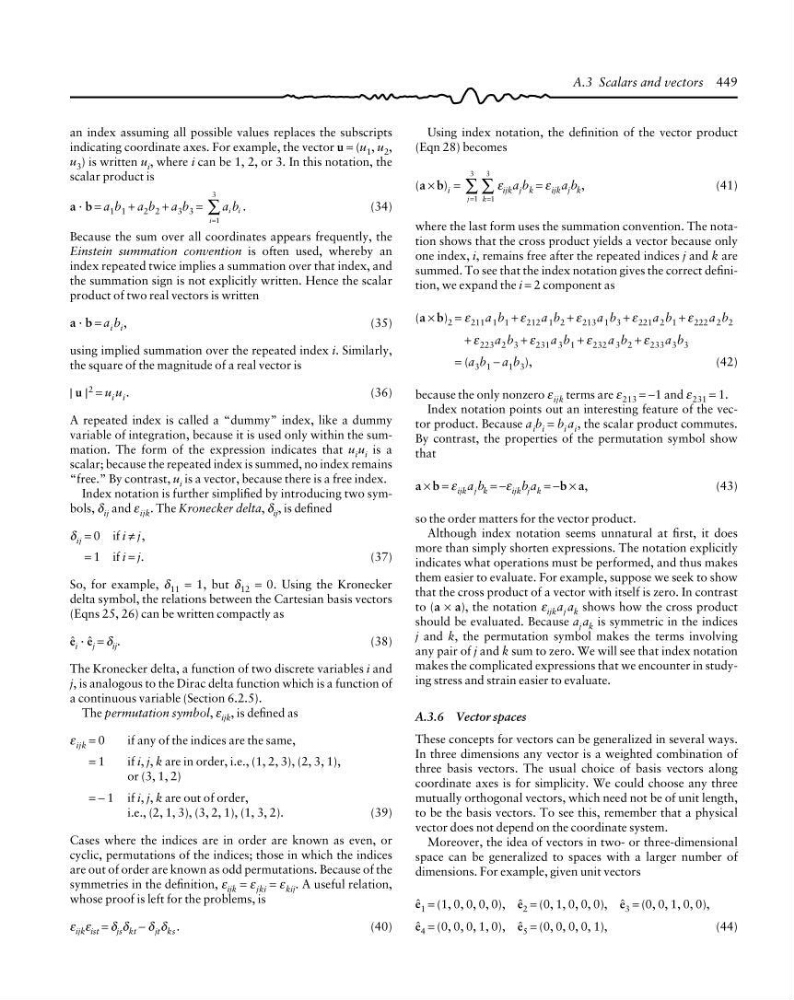
an index assuming all possible values replaces the subscripts
indicating coordinate axes. For example, the vector u = (u 1 , u 2 ,
u 3 ) is written u i , where i can be 1, 2, or 3. In this notation, the
scalar product is
a · b = a 1 b 1 + a 2 b 2 + a 3 b 3 =
a b
i i
i=
∑
1
3
.
(34)
Because the sum over all coordinates appears frequently, the
Einstein summation convention is often used, whereby an
index repeated twice implies a summation over that index, and
the summation sign is not explicitly written. Hence the scalar
product of two real vectors is written
a · b = a i b i ,
(35)
using implied summation over the repeated index i. Similarly,
the square of the magnitude of a real vector is
| u | 2 = u i u i .
(36)
A repeated index is called a “dummy” index, like a dummy
variable of integration, because it is used only within the summation. The form of the expression indicates that u i u i is a
scalar; because the repeated index is summed, no index remains
“free.” By contrast, u i is a vector, because there is a free index.
Index notation is further simplified by introducing two symbols, δ ij and ε ijk . The Kronecker delta, δ ij , is defined
δ ij = 0 if i ≠ j,
= 1 if i = j.
(37)
So, for example, δ 11 = 1, but δ 12 = 0. Using the Kronecker
delta symbol, the relations between the Cartesian basis vectors
(Eqns 25, 26) can be written compactly as
ê i · ê j = δ ij .
(38)
The Kronecker delta, a function of two discrete variables i and
j, is analogous to the Dirac delta function which is a function of
a continuous variable (Section 6.2.5).
The permutation symbol, ε ijk , is defined as
ε ijk = 0
if any of the indices are the same,
= 1
if i, j, k are in order, i.e., (1, 2, 3), (2, 3, 1),
or (3, 1, 2)
= − 1 if i, j, k are out of order,
i.e., (2, 1, 3), (3, 2, 1), (1, 3, 2).
(39)
Cases where the indices are in order are known as even, or
cyclic, permutations of the indices; those in which the indices
are out of order are known as odd permutations. Because of the
symmetries in the definition, ε ijk = ε jki = ε kij . A useful relation,
whose proof is left for the problems, is
ε ijk ε ist = δ js δ kt − δ jt δ ks .
(40)
Using index notation, the definition of the vector product
(Eqn 28) becomes
(a × b) i =
j
k
=
=
∑ ∑
1
3
1
3
ε ijk a j b k = ε ijk a j b k ,
(41)
where the last form uses the summation convention. The notation shows that the cross product yields a vector because only
one index, i, remains free after the repeated indices j and k are
summed. To see that the index notation gives the correct definition, we expand the i = 2 component as
(a × b) 2 = ε 211 a 1 b 1 + ε 212 a 1 b 2 + ε 213 a 1 b 3 + ε 221 a 2 b 1 + ε 222 a 2 b 2
+ ε 223 a 2 b 3 + ε 231 a 3 b 1 + ε 232 a 3 b 2 + ε 233 a 3 b 3
= (a 3 b 1 − a 1 b 3 ),
(42)
because the only nonzero ε ijk terms are ε 213 = −1 and ε 231 = 1.
Index notation points out an interesting feature of the vector product. Because a i b i = b i a i , the scalar product commutes.
By contrast, the properties of the permutation symbol show
that
a × b = ε ijk a j b k = −ε ijk b j a k = −b × a,
(43)
so the order matters for the vector product.
Although index notation seems unnatural at first, it does
more than simply shorten expressions. The notation explicitly
indicates what operations must be performed, and thus makes
them easier to evaluate. For example, suppose we seek to show
that the cross product of a vector with itself is zero. In contrast
to (a × a), the notation ε ijk a j a k shows how the cross product
should be evaluated. Because a j a k is symmetric in the indices
j and k, the permutation symbol makes the terms involving
any pair of j and k sum to zero. We will see that index notation
makes the complicated expressions that we encounter in studying stress and strain easier to evaluate.
A.3.6 Vector spaces
These concepts for vectors can be generalized in several ways.
In three dimensions any vector is a weighted combination of
three basis vectors. The usual choice of basis vectors along
coordinate axes is for simplicity. We could choose any three
mutually orthogonal vectors, which need not be of unit length,
to be the basis vectors. To see this, remember that a physical
vector does not depend on the coordinate system.
Moreover, the idea of vectors in two- or three-dimensional
space can be generalized to spaces with a larger number of
dimensions. For example, given unit vectors
ê 1 = (1, 0, 0, 0, 0), ê 2 = (0, 1, 0, 0, 0), ê 3 = (0, 0, 1, 0, 0),
ê 4 = (0, 0, 0, 1, 0), ê 5 = (0, 0, 0, 0, 1),
(44)
A.3 Scalars and vectors 449
indicating coordinate axes. For example, the vector u = (u 1 , u 2 ,
u 3 ) is written u i , where i can be 1, 2, or 3. In this notation, the
scalar product is
a · b = a 1 b 1 + a 2 b 2 + a 3 b 3 =
a b
i i
i=
∑
1
3
.
(34)
Because the sum over all coordinates appears frequently, the
Einstein summation convention is often used, whereby an
index repeated twice implies a summation over that index, and
the summation sign is not explicitly written. Hence the scalar
product of two real vectors is written
a · b = a i b i ,
(35)
using implied summation over the repeated index i. Similarly,
the square of the magnitude of a real vector is
| u | 2 = u i u i .
(36)
A repeated index is called a “dummy” index, like a dummy
variable of integration, because it is used only within the summation. The form of the expression indicates that u i u i is a
scalar; because the repeated index is summed, no index remains
“free.” By contrast, u i is a vector, because there is a free index.
Index notation is further simplified by introducing two symbols, δ ij and ε ijk . The Kronecker delta, δ ij , is defined
δ ij = 0 if i ≠ j,
= 1 if i = j.
(37)
So, for example, δ 11 = 1, but δ 12 = 0. Using the Kronecker
delta symbol, the relations between the Cartesian basis vectors
(Eqns 25, 26) can be written compactly as
ê i · ê j = δ ij .
(38)
The Kronecker delta, a function of two discrete variables i and
j, is analogous to the Dirac delta function which is a function of
a continuous variable (Section 6.2.5).
The permutation symbol, ε ijk , is defined as
ε ijk = 0
if any of the indices are the same,
= 1
if i, j, k are in order, i.e., (1, 2, 3), (2, 3, 1),
or (3, 1, 2)
= − 1 if i, j, k are out of order,
i.e., (2, 1, 3), (3, 2, 1), (1, 3, 2).
(39)
Cases where the indices are in order are known as even, or
cyclic, permutations of the indices; those in which the indices
are out of order are known as odd permutations. Because of the
symmetries in the definition, ε ijk = ε jki = ε kij . A useful relation,
whose proof is left for the problems, is
ε ijk ε ist = δ js δ kt − δ jt δ ks .
(40)
Using index notation, the definition of the vector product
(Eqn 28) becomes
(a × b) i =
j
k
=
=
∑ ∑
1
3
1
3
ε ijk a j b k = ε ijk a j b k ,
(41)
where the last form uses the summation convention. The notation shows that the cross product yields a vector because only
one index, i, remains free after the repeated indices j and k are
summed. To see that the index notation gives the correct definition, we expand the i = 2 component as
(a × b) 2 = ε 211 a 1 b 1 + ε 212 a 1 b 2 + ε 213 a 1 b 3 + ε 221 a 2 b 1 + ε 222 a 2 b 2
+ ε 223 a 2 b 3 + ε 231 a 3 b 1 + ε 232 a 3 b 2 + ε 233 a 3 b 3
= (a 3 b 1 − a 1 b 3 ),
(42)
because the only nonzero ε ijk terms are ε 213 = −1 and ε 231 = 1.
Index notation points out an interesting feature of the vector product. Because a i b i = b i a i , the scalar product commutes.
By contrast, the properties of the permutation symbol show
that
a × b = ε ijk a j b k = −ε ijk b j a k = −b × a,
(43)
so the order matters for the vector product.
Although index notation seems unnatural at first, it does
more than simply shorten expressions. The notation explicitly
indicates what operations must be performed, and thus makes
them easier to evaluate. For example, suppose we seek to show
that the cross product of a vector with itself is zero. In contrast
to (a × a), the notation ε ijk a j a k shows how the cross product
should be evaluated. Because a j a k is symmetric in the indices
j and k, the permutation symbol makes the terms involving
any pair of j and k sum to zero. We will see that index notation
makes the complicated expressions that we encounter in studying stress and strain easier to evaluate.
A.3.6 Vector spaces
These concepts for vectors can be generalized in several ways.
In three dimensions any vector is a weighted combination of
three basis vectors. The usual choice of basis vectors along
coordinate axes is for simplicity. We could choose any three
mutually orthogonal vectors, which need not be of unit length,
to be the basis vectors. To see this, remember that a physical
vector does not depend on the coordinate system.
Moreover, the idea of vectors in two- or three-dimensional
space can be generalized to spaces with a larger number of
dimensions. For example, given unit vectors
ê 1 = (1, 0, 0, 0, 0), ê 2 = (0, 1, 0, 0, 0), ê 3 = (0, 0, 1, 0, 0),
ê 4 = (0, 0, 0, 1, 0), ê 5 = (0, 0, 0, 0, 1),
(44)
A.3 Scalars and vectors 449