

30 Basic Seismological Theory
y
x
u(x + dx, t)
τ
θ 2
θ
θ 1
θ
u(x, t)
du
dx
τ
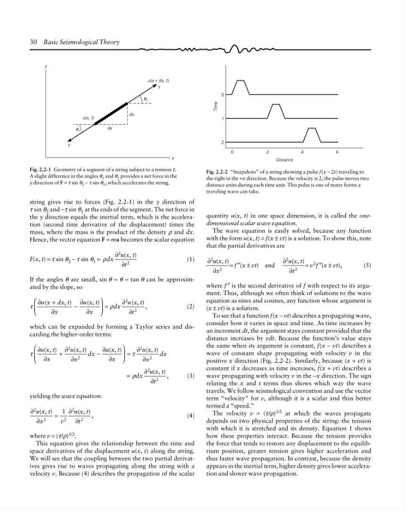
Fig. 2.2-1 Geometry of a segment of a string subject to a tension τ.
A slight difference in the angles θ 1 and θ 2 provides a net force in the
y direction of F = τ sin θ 2 − τ sin θ 1 , which accelerates the string.
Time
0
1
2
0
Distance
2
4
6
Fig. 2.2-2 “Snapshots” of a string showing a pulse f(x − 2t) traveling to
the right in the +x direction. Because the velocity is 2, the pulse moves two
distance units during each time unit. This pulse is one of many forms a
traveling wave can take.
string gives rise to forces (Fig. 2.2-1) in the y direction of
τ sin θ 2 and −τ sin θ 1 at the ends of the segment. The net force in
the y direction equals the inertial term, which is the acceleration (second time derivative of the displacement) times the
mass, where the mass is the product of the density ρ and dx.
Hence, the vector equation F = ma becomes the scalar equation
F(x, t) = τ sin θ 2 − τ sin θ 1 = ρdx
u x t
t
∂
∂
2
2
( , )
(1)
If the angles θ are small, sin θ ≈ θ ≈ tan θ can be approximated by the slope, so
τ
ρ
∂
+
∂
−
∂
∂
⎛
⎝
⎜
⎞
⎠
⎟ =
∂
∂
u x dx t
x
u x t
x
dx
u x t
t
(
, )
( , )
( , ) ,
2
2
(2)
which can be expanded by forming a Taylor series and discarding the higher-order terms:
τ
τ
∂
∂
+
∂
∂
−
∂
∂
⎛
⎝
⎜
⎞
⎠
⎟ =
∂
∂
u x t
x
u x t
x
dx
u x t
x
u x t
x
dx
( , )
( , )
( , )
( , )
2
2
2
2
=
∂
∂
( , ) ,
ρdx
u x t
t
2
2
(3)
yielding the wave equation:
∂
∂
=
∂
∂
2
2
2
2
2
1
u x t
x
v
u x t
t
( , )
( , ) ,
(4)
where v = (τ/ρ)
1/2
.
This equation gives the relationship between the time and
space derivatives of the displacement u(x, t) along the string.
We will see that the coupling between the two partial derivatives gives rise to waves propagating along the string with a
velocity v. Because (4) describes the propagation of the scalar
quantity u(x, t) in one space dimension, it is called the onedimensional scalar wave equation.
The wave equation is easily solved, because any function
with the form u(x, t) = f(x ± vt) is a solution. To show this, note
that the partial derivatives are
∂
∂
2
2
u x t
x
( , ) = f ″(x ± vt) and
∂
∂
2
2
u x t
t
( , ) = v 2 f ″(x ± vt),
(5)
where f ″ is the second derivative of f with respect to its argument. Thus, although we often think of solutions to the wave
equation as sines and cosines, any function whose argument is
(x ± vt) is a solution.
To see that a function f(x − vt) describes a propagating wave,
consider how it varies in space and time. As time increases by
an increment dt, the argument stays constant provided that the
distance increases by vdt. Because the function’s value stays
the same when its argument is constant, f(x − vt) describes a
wave of constant shape propagating with velocity v in the
positive x direction (Fig. 2.2-2). Similarly, because (x + vt) is
constant if x decreases as time increases, f(x + vt) describes a
wave propagating with velocity v in the −x direction. The sign
relating the x and t terms thus shows which way the wave
travels. We follow seismological convention and use the vector
term “velocity” for v, although it is a scalar and thus better
termed a “speed.”
The velocity v = (τ/ρ) 1/2 at which the waves propagate
depends on two physical properties of the string: the tension
with which it is stretched and its density. Equation 1 shows
how these properties interact. Because the tension provides
the force that tends to restore any displacement to the equilibrium position, greater tension gives higher acceleration and
thus faster wave propagation. In contrast, because the density
appears in the inertial term, higher density gives lower acceleration and slower wave propagation.
y
x
u(x + dx, t)
τ
θ 2
θ
θ 1
θ
u(x, t)
du
dx
τ
Fig. 2.2-1 Geometry of a segment of a string subject to a tension τ.
A slight difference in the angles θ 1 and θ 2 provides a net force in the
y direction of F = τ sin θ 2 − τ sin θ 1 , which accelerates the string.
Time
0
1
2
0
Distance
2
4
6
Fig. 2.2-2 “Snapshots” of a string showing a pulse f(x − 2t) traveling to
the right in the +x direction. Because the velocity is 2, the pulse moves two
distance units during each time unit. This pulse is one of many forms a
traveling wave can take.
string gives rise to forces (Fig. 2.2-1) in the y direction of
τ sin θ 2 and −τ sin θ 1 at the ends of the segment. The net force in
the y direction equals the inertial term, which is the acceleration (second time derivative of the displacement) times the
mass, where the mass is the product of the density ρ and dx.
Hence, the vector equation F = ma becomes the scalar equation
F(x, t) = τ sin θ 2 − τ sin θ 1 = ρdx
u x t
t
∂
∂
2
2
( , )
(1)
If the angles θ are small, sin θ ≈ θ ≈ tan θ can be approximated by the slope, so
τ
ρ
∂
+
∂
−
∂
∂
⎛
⎝
⎜
⎞
⎠
⎟ =
∂
∂
u x dx t
x
u x t
x
dx
u x t
t
(
, )
( , )
( , ) ,
2
2
(2)
which can be expanded by forming a Taylor series and discarding the higher-order terms:
τ
τ
∂
∂
+
∂
∂
−
∂
∂
⎛
⎝
⎜
⎞
⎠
⎟ =
∂
∂
u x t
x
u x t
x
dx
u x t
x
u x t
x
dx
( , )
( , )
( , )
( , )
2
2
2
2
=
∂
∂
( , ) ,
ρdx
u x t
t
2
2
(3)
yielding the wave equation:
∂
∂
=
∂
∂
2
2
2
2
2
1
u x t
x
v
u x t
t
( , )
( , ) ,
(4)
where v = (τ/ρ)
1/2
.
This equation gives the relationship between the time and
space derivatives of the displacement u(x, t) along the string.
We will see that the coupling between the two partial derivatives gives rise to waves propagating along the string with a
velocity v. Because (4) describes the propagation of the scalar
quantity u(x, t) in one space dimension, it is called the onedimensional scalar wave equation.
The wave equation is easily solved, because any function
with the form u(x, t) = f(x ± vt) is a solution. To show this, note
that the partial derivatives are
∂
∂
2
2
u x t
x
( , ) = f ″(x ± vt) and
∂
∂
2
2
u x t
t
( , ) = v 2 f ″(x ± vt),
(5)
where f ″ is the second derivative of f with respect to its argument. Thus, although we often think of solutions to the wave
equation as sines and cosines, any function whose argument is
(x ± vt) is a solution.
To see that a function f(x − vt) describes a propagating wave,
consider how it varies in space and time. As time increases by
an increment dt, the argument stays constant provided that the
distance increases by vdt. Because the function’s value stays
the same when its argument is constant, f(x − vt) describes a
wave of constant shape propagating with velocity v in the
positive x direction (Fig. 2.2-2). Similarly, because (x + vt) is
constant if x decreases as time increases, f(x + vt) describes a
wave propagating with velocity v in the −x direction. The sign
relating the x and t terms thus shows which way the wave
travels. We follow seismological convention and use the vector
term “velocity” for v, although it is a scalar and thus better
termed a “speed.”
The velocity v = (τ/ρ) 1/2 at which the waves propagate
depends on two physical properties of the string: the tension
with which it is stretched and its density. Equation 1 shows
how these properties interact. Because the tension provides
the force that tends to restore any displacement to the equilibrium position, greater tension gives higher acceleration and
thus faster wave propagation. In contrast, because the density
appears in the inertial term, higher density gives lower acceleration and slower wave propagation.